Lab 9: Linear regression#
Simple linear regression#
Simulating linear regression data#
x = rnorm(100, mean=3, sd=1)
error = rnorm(100, mean=0, sd=2)
y = 2.1+1.25*x+error

data=data.frame(cbind(x,y))
Fitting the linear regression model#
result = lm(data$y~data$x)
summary(result)
Call:
lm(formula = data$y ~ data$x)

Residuals:
   Min     1Q Median     3Q    Max
-4.492 -1.564  0.035  1.184  6.029

Coefficients:
            Estimate Std. Error t value Pr(>|t|)
(Intercept)   3.3126     0.6830   4.850 4.64e-06 ***
data$x        0.8620     0.2122   4.062 9.82e-05 ***
---
Signif. codes:  0 ‘***’ 0.001 ‘**’ 0.01 ‘*’ 0.05 ‘.’ 0.1 ‘ ’ 1

Residual standard error: 1.962 on 98 degrees of freedom
Multiple R-squared:  0.1441,	Adjusted R-squared:  0.1354
F-statistic:  16.5 on 1 and 98 DF,  p-value: 9.818e-05
Residual plot#
par(mfrow=c(2,2))
plot(x,y,pch=16)
abline(result,col="brown")
plot(result$residuals)
abline(a=0,b=0, col="brown")
hist(result$residuals)
qqnorm(result$residuals, pch=16)
qqline(result$residuals, col = "brown")
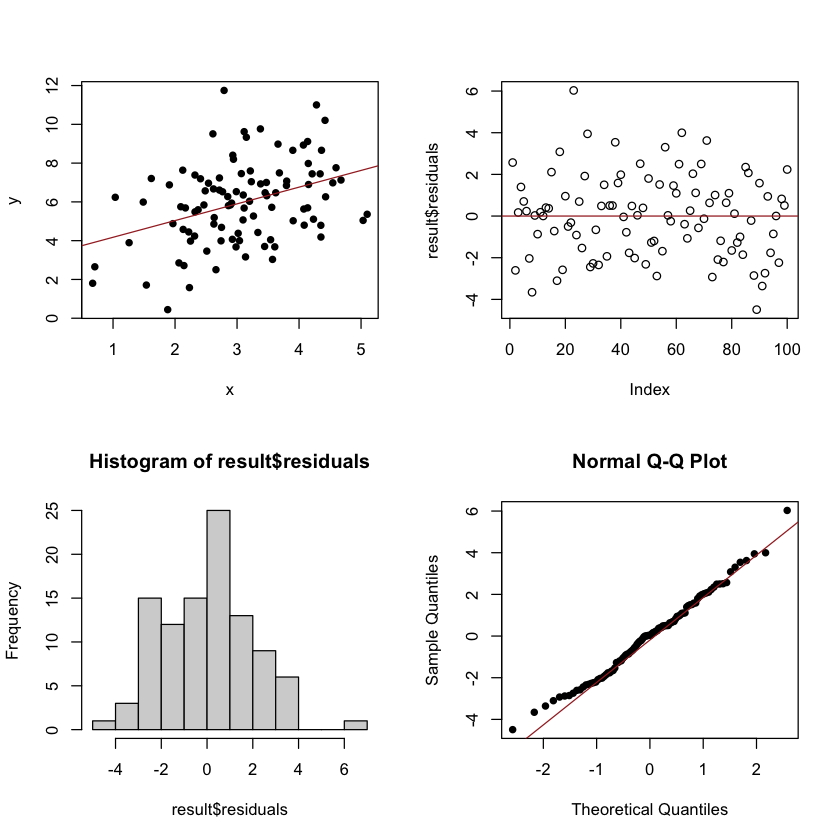
Checking normality#
shapiro.test(result$residuals)
	Shapiro-Wilk normality test

data:  result$residuals
W = 0.99047, p-value = 0.7028
Prediction for new observations#
x_new = 0.7
y_new = result$coefficients[1]+result$coefficients[2]*x_new
y_new
(Intercept): 3.91606027399812
Fitting quadratic relationships#
x = rnorm(100, mean=0, sd=1)
y = 2.1+1.25*x^2+error
data=data.frame(cbind(x,y))
result = lm(data$y~data$x)
summary(result)
Call:
lm(formula = data$y ~ data$x)

Residuals:
    Min      1Q  Median      3Q     Max
-4.6360 -1.5817 -0.0843  1.5278  8.2568

Coefficients:
            Estimate Std. Error t value Pr(>|t|)
(Intercept)   3.2918     0.2470  13.327   <2e-16 ***
data$x       -0.4565     0.2494  -1.831   0.0702 .
---
Signif. codes:  0 ‘***’ 0.001 ‘**’ 0.01 ‘*’ 0.05 ‘.’ 0.1 ‘ ’ 1

Residual standard error: 2.454 on 98 degrees of freedom
Multiple R-squared:  0.03306,	Adjusted R-squared:  0.02319
F-statistic: 3.351 on 1 and 98 DF,  p-value: 0.07021
Multiple linear regression#
Generating data#
x1 = rnorm(100, mean=3, sd=1)
x2 = rnorm(100, mean=2.5, sd=2.1)

error = rnorm(100, mean=0, sd=2)
y = 2.1 + 1.25*x1 - 3*x2 + error

data=data.frame(cbind(y,x1,x2))
plot(data)

Fitting the model#
result = lm(y~x1+x2,data=data)
summary(result)
Call:
lm(formula = y ~ x1 + x2, data = data)

Residuals:
    Min      1Q  Median      3Q     Max
-4.8136 -1.5113  0.0226  1.4080  5.0071

Coefficients:
            Estimate Std. Error t value Pr(>|t|)
(Intercept)   1.3971     0.7364   1.897   0.0608 .
x1            1.3777     0.2347   5.870 6.08e-08 ***
x2           -2.8028     0.1018 -27.523  < 2e-16 ***
---
Signif. codes:  0 ‘***’ 0.001 ‘**’ 0.01 ‘*’ 0.05 ‘.’ 0.1 ‘ ’ 1

Residual standard error: 2.022 on 97 degrees of freedom
Multiple R-squared:  0.8898,	Adjusted R-squared:  0.8876
F-statistic: 391.8 on 2 and 97 DF,  p-value: < 2.2e-16
Residual plot#
par(mfrow=c(2,2))
plot(result$residuals)
abline(a=0,b=0, col="red")
hist(result$residuals)
qqnorm(result$residuals, pch=16)
qqline(result$residuals, col = "brown")
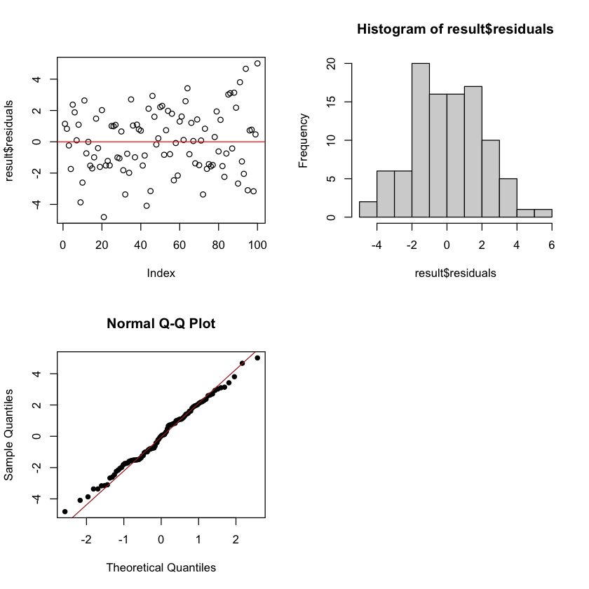
Checking the normality assumption#
shapiro.test(result$residuals)
	Shapiro-Wilk normality test

data:  result$residuals
W = 0.99217, p-value = 0.8337
Logistic regression#
Generating data#
age <- round(runif(100, 18, 80))
log_odds = -2.2 + 0.02*age
p = 1/(1 + exp(-log_odds))
y <- rbinom(n = 100, size = 1, prob = p)
Fitting the logistic model#
mod <- glm(y ~ age, family = "binomial")
summary(mod)
Call:
glm(formula = y ~ age, family = "binomial")

Deviance Residuals:
    Min       1Q   Median       3Q      Max
-1.0593  -0.7440  -0.5259  -0.3979   2.2962

Coefficients:
            Estimate Std. Error z value Pr(>|z|)
(Intercept) -3.27148    0.86797  -3.769 0.000164 ***
age          0.03734    0.01500   2.490 0.012787 *
---
Signif. codes:  0 ‘***’ 0.001 ‘**’ 0.01 ‘*’ 0.05 ‘.’ 0.1 ‘ ’ 1

(Dispersion parameter for binomial family taken to be 1)

    Null deviance: 102.791  on 99  degrees of freedom
Residual deviance:  95.974  on 98  degrees of freedom
AIC: 99.974

Number of Fisher Scoring iterations: 4