Chapter 0: Prerequisites#
“Do the difficult things while they are easy and do the great things while they are small. A journey of a thousand miles must begin with a single step.”
—Lao Tzu
See also
Calculus#
Derivative#
Definition (derivative)
The derivative \(f^{\prime}(x)\) of a differentiable function \(f(x)\) at \(x\) is defined as the limit
The derivative \(f^{\prime}(a)\) is the instantaneous rate of change of \(y=f(x)\) at \(x=a\). If \(f(x)\) is the position of an object at time \(x\) then the derivate \(f^{\prime}(a)\) is the velocity of the object at \(x=a\).
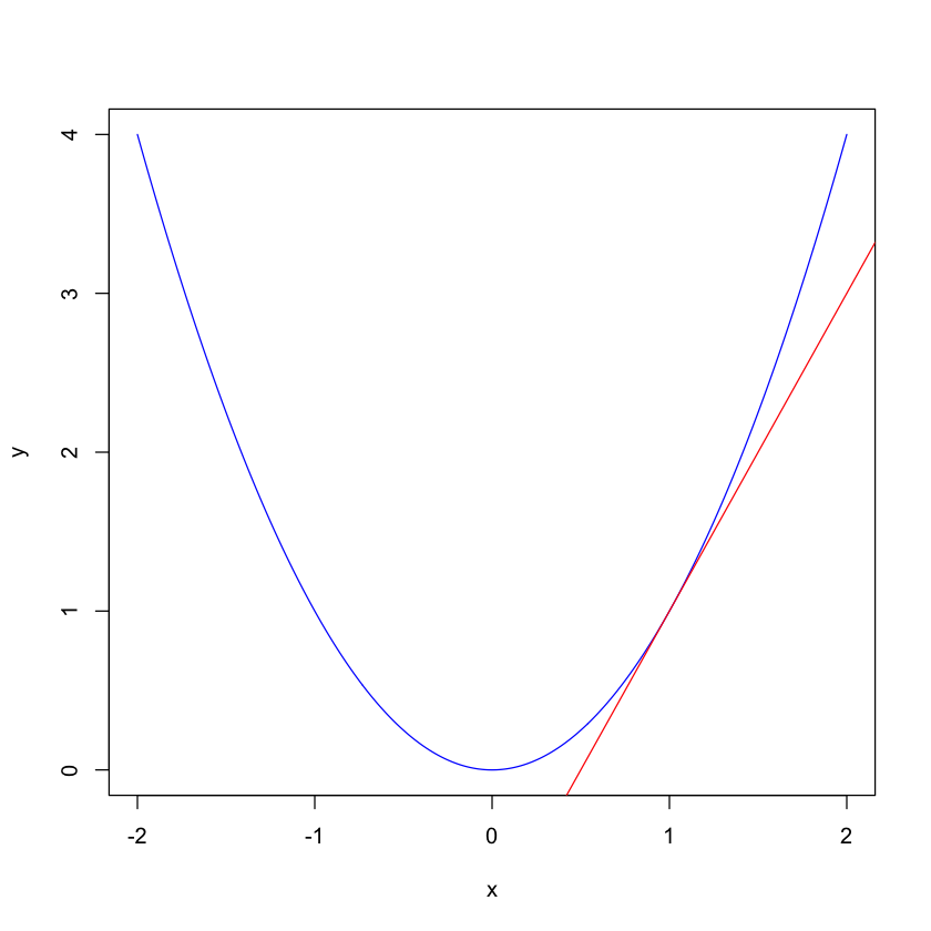
Geometrically, the derivate of \(f(x)\) at \(x=a\) is the slope of the tangent line of the graph \(y=f(x)\) at \(x=a\). The equation of the tangent line is given by
A function \(f(x)\) is said to be differentiable at \(x=a\) if the derivative \(f^{\prime}(a)\) exists. If \(f(x)\) is differentiable at any point in an open set \(D\subset\mathbb{R}\), we say that \(f(x)\) is differentiable on \(D\).
x = seq(-2,2,by=0.01)
y = x^2
plot(x,y,type="l",col="blue")
abline(a=-1,b=2,col="red")
Notation
If \(y=f(x)\), then all of the following are equivalent notations for the derivative. \(f^{\prime}(x)=y^{\prime}=\frac{d f}{d x}=\frac{d y}{d x}=\frac{d}{d x}(f(x))=D_xf\)
If \(y=f(x)\), then all of the following are equivalent notations for derivative evaluated at \(x=a\). \(f^{\prime}(a)=\left.y^{\prime}\right|_{x=a}=\left.\frac{d f}{d x}\right|_{x=a}=\left.\frac{d y}{d x}\right|_{x=a}=D_af\)
Note that if \(f\) is a constant function, then its derivative is equal to 0.
Theorem 1 (linearity of derivative)
Given two functions \(f\) and \(g\) that are differentiable at a point \(a\), the derivate of the sum of two functions is equal to the sum of the derivatives of two functions, i.e.,
Suppose \(c\) is a real number, then
The product rule: \((f g)^{\prime}=f^{\prime} g+f g^{\prime}\)
The quotient rule: \(\left(\frac{f}{g}\right)^{\prime}=\frac{f^{\prime} g-f g^{\prime}}{g^{2}}\)
The power rule: \(\frac{d}{d x}\left(x^{n}\right)=n x^{n-1}\)
The chain rule: \(\frac{d}{d x}(f(g(x)))=f^{\prime}(g(x)) g^{\prime}(x)\)
Common Derivatives
\((x)^{\prime}=1\)
\(\left(x^n\right)^{\prime} = nx^{n-1}\)
\(\left(a^{x}\right)^\prime=a^{x} \ln (a)\)
\(\left(e^x\right)^\prime=e^x\)
\((\ln x)^\prime=\frac{1}{x}\)
\((\sin x)^\prime=\cos x\)
\((\cos x)^\prime=-\sin x\)
par(mfrow=c(2,2))
#polynomial
x = seq(-10,10,0.01)
y = x^3
plot(x,y,type="l",col="blue",main="polynomial")

#exponential
x = seq(-10,10,0.01)
y = exp(x)
plot(x,y,type="l",col="blue",main="exponential")

#logrithm
x = seq(0.01,10,0.01)
y = log(x)
plot(x,y,type="l",col="blue",main="log")

#trig
x = seq(-10,10,0.01)
y = sin(x)
plot(x,y,type="l",col="blue",main="sin")

Example (0.1)
Find the derivative \(\frac{de^{2x}}{dx}\)
Let \(y=2x\) and by the chain rule we have \(\frac{de^{2x}}{dx}=\frac{(de^y)}{dy}\frac{dy}{dx}=e^{y}*2=2e^{2x}\)
Derivatives can be used to minimize or maximize a differentiable function \(f(x)\). To find the value of \(x\) that can maximize or minimize the function \(f(x)\), we set the first derivative to be 0, i.e., \(f^{\prime}(x)=0\) and check the second derivative of \(f(x)\).
Example (0.2)
Find the value of \(x\) that can minimize \(f(x)=x^2\) Set the first derivate to be 0, i.e., \(f^{\prime}(x)=0\), which indicates that \(2x=0\) or \(x=0\). Since the second derivative \(f^{''} (x)=2\) is greater than 0, the value \(x=0\) minimizes the function \(f(x)=x^2\).
Integral#
Theorem 2 (Fundamental Theorem of Calculus)
If \(F(x)\) is an anti-derivative of \(f(x)\), then
Common Integrals
\(\int k d x=k x+c\)
\(\int x^{n} d x=\frac{1}{n+1} x^{n+1}+c\)
\(\int \sin u d u=-\cos u+c\)
\(\int \cos u d u=\sin u+c\)
\(\int x^{-1} d x=\int \frac{1}{x} d x=\ln |x|+c\)
\(\int \frac{1}{a x+b} d x=\frac{1}{a} \ln |a x+b|+c\)
\(\int \ln u d u=u \ln (u)-u+c\)
\(\int e^u du=e^u+c\)
\(\int \frac{1}{a^{2}+u^{2}} d u=\frac{1}{a} \tan ^{-1}\left(\frac{u}{a}\right)+c\)
\(\int \frac{1}{\sqrt{a^{2}-u^{2}}} d u=\sin ^{-1}\left(\frac{u}{a}\right)+c\)
Approximation#
The continuous functions can be approximated by polynomial functions, which is called Taylor series. The Taylor series to a smooth function \(f(x)\) near \(x=a\) is
Example (0.3)
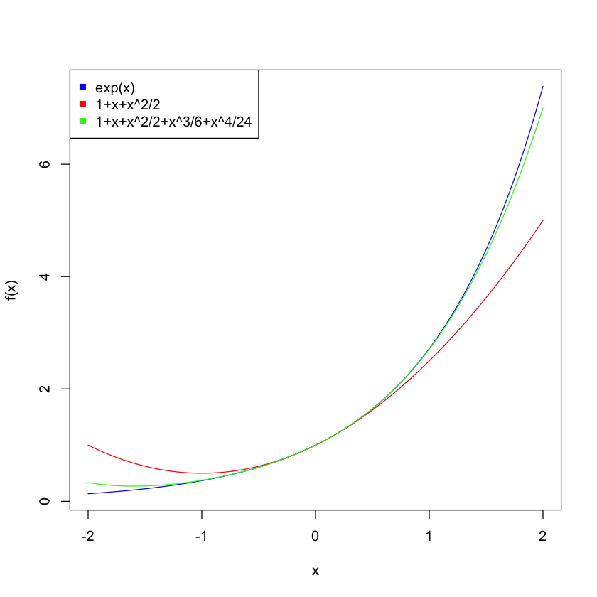
Find the Taylor series of \(f(x)=e^x\) near \(x=0\)
Because \(a=0\), \(f(a)=e^a=e^0=1\) and \(f^n(a)=e^0=1\). It follows from the above equation that the Taylor series of \(e^x\) near \(x=0\) is given by
Show code cell source
x = seq(-2,2,0.01)
y1 = exp(x)
y2 = 1 + x + x^2/2
y3 = 1 + x + x^2/2 + x^3/6 + x^4/24

plot(x,y1,type="l",ylab="f(x)",col="blue")
lines(x,y2,col="red")
lines(x,y3,col="green")
legend("topleft",legend=c("exp(x)","1+x+x^2/2","1+x+x^2/2+x^3/6+x^4/24"),col=c("blue","red","green"),pch=15)
Linear algebra#
Dot product#
Definition (dot product)
The dot product of two vectors \(a=(a_1,…,a_n)\) and \(b=(b_1,…,b_n)\) is given by
Example (0.4)
The dot product of two vectors \((1, 2, 3)\) and \((0, 1, 2)\) is \(1*0+2*1+3*2=8\). Note that two vectors must have the same length.
Definition (orthogonal)
Two vectors \(a=(a_1,…,a_n)\) and \(b=(b_1,…,b_n)\) are orthogonal (perpendicular) if \(a\cdot b=0\).
Example (0.5)
Two vectors \((0, 1)\) and \((1, 0)\) are orthogonal because their dot product is equal to 0, i.e., \((0, 1)\cdot (1, 0) = 0\)
Matrices multiplication: \(A_{n×k} B_{k×m}=C_{n×m}\), in which \(c_{ij}=∑_{w=1}^ka_{iw} b_{wj} \).
Linear independent#
Definition (linear dependent)
Let \(\left(a_1,\dots,a_n\right)\) denote the \(n\) column vectors of matrix \(A\). Those vectors are linearly dependent if and only if there is a non-zero vector \((x_1,\dots,x_n)\) such that
In the matrix \(A=\begin{pmatrix} 1&2\\1&2\end{pmatrix}\), the column vectors \((1, 1)\) and \((2, 2)\) are linearly dependent because \(2*(1, 1)-(2, 2) = 0\).
The column vectors are linearly independent if and only if the zero vector is the only solution to \(x_1 a_1+\dots+x_n a_n=0\).
Example (0.6)
In the matrix \(A=\begin{pmatrix} 1&0\\0&1\end{pmatrix}\), the column vectors \((1, 0)\) and \((0, 1)\) are linearly independent, because if \(x_1 (1, 0)+x_2 (0, 1)=(0, 0)\), then \(x_1=0\) and \(x_2=0\).
Basis#
Definition (basis)
A set of vectors in a vector space \(V\) is called a basis, or a set of basis vectors, if the vectors are linearly independent and every vector in the vector space is a linear combination of this set.
For example, the basis of a two-dimensional space could be \((0, 1)\) and \((1, 0)\). It is easy to check that \((0, 1)\) and \((1, 0)\) are linearly independent and every vector \((x, y)\) is a linear combination of two basis vectors, i.e., \((x, y)=x(1, 0)+y(0, 1)\).
The basis vectors are not unique, for example, \((-1, 1)\) and \((1, 1)\) are basis vectors because they are linearly independent and every vector in the two-dimensional space is a linear combination of \((-1, 1)\) and \((1, 1)\). In fact, any two linearly independent vectors are the basis of the two-dimensional space.
It can be shown that the \(n\) dimensional space has \(n\) basis vectors.
The rank of a matrix = the number of linearly independent column vectors
The inverse of a matrix \(A\). If we can find a matrix \(B\) such that \(AB=I\) (identity matrix), matrix \(B\) is the inverse of matrix \(A\). The inverse of matrix \(A\) is often represented by \(A^{-1}\).
Determinant of a square matrix \(A\), denoted by \(\det(A)\) or \(|A|\). The matrix \(A\) has a unique inverse if and only if its determinant is not \(0\).
Eigenvector#
Definition (eigenvector)
Let \(A\) be a square matrix. If we can find a non-zero vector \(x\) and a number \(\lambda\) such that \(Ax=\lambda x\), the vector \(x\) is an eigenvector and the number \(\lambda\) is an eigenvalue.
We need to find \(x\) and \(\lambda\) such that \((A-\lambda I)x=0\). Since \(x\) is a non-zero vector, it indicates that \(A-λI\) is not invertible, i.e., \(\det(A-\lambda I)=0\).
Definition (diagonalizable)
A square matrix \(A\) is diagonalizable if it can be written as \(A=PDP^{-1}\), in which the column vectors of \(P\) are eigenvectors of \(A\) and \(D\) is a diagonal matrix of eigenvalues.
If a square matrix \(A\) is diagonalizable, then it is straightforward to calculate \(A^2\),
Statistics#
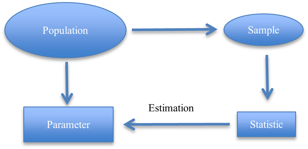
The ultimate goal of statistical inference is to understand the unknown population through the samples generated from the population. The population is characterized by so called parameters. We often calculate statistics from samples to estimate parameters.
Example (0.7)
We want to know the average weight of UGA students. We take a random sample of 100 students and calculate their average weight, which is 135 pounds. We conclude that the average weight of UGA students is 135 pounds.
Population: the weights of all UGA students
Parameter: the mean weight or the population mean
Sample: 100 students’ weights
Statistic: the average weight of the sample or the sample average
We use the sample average to estimate the population mean. Does it make sense? What is the probability that the population mean is exactly equal to 135 pounds? How do we handle uncertainty?
Converting a real problem to a mathematical problem
How do we denote a population in math? The population is represented by a probability distribution \(f(x \mid \theta)\) where \(\theta\) is the population parameter and \(x\) is the random variable of interest. In the above example, the random variable \(x\) denotes the weight of an individual randomly selected from the population. In other words, the probability distribution function \(f(x|\theta)\) represents how the weight is distributed in the population.
How do we denote parameter in math? The parameter is a constant \(\theta\) characterizing the population. For example, the parameter of a population includes the population mean, the population variance, the population median, etc.
How do we denote a sample in math? The observations in a sample are random numbers generated from the probability distribution, i.e., \(\boldsymbol{x}_{\mathbf{1}}, \ldots, \boldsymbol{x}_{\boldsymbol{n}} \sim \boldsymbol{f}(\boldsymbol{x} \mid \boldsymbol{\theta})\)
How do we denote a statistic in math? A statistic is a function of the sample.
Important conclusions
If we know the population, i.e., the probability distribution, we do not need to generate real data in the wet lab. We can use computers to simulate data from the probability distribution.
If we have data, we can make inference about the population (i.e., the probability distribution) from data.