Chapter 12: Bayesian analysis#
“Do the difficult things while they are easy and do the great things while they are small. A journey of a thousand miles must begin with a single step.”
—Lao Tzu
See also
In the Bayesian framework, probability is considered as an expression of opinion, and the process of drawing inferences from data is essentially the revision of this opinion in response to pertinent new information.
Example 71
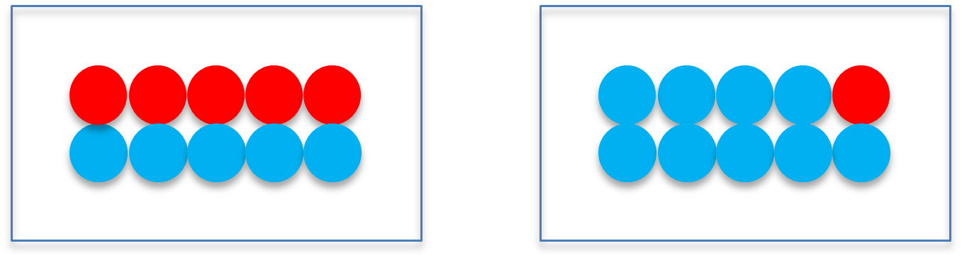
There are two boxes in the room: Box 1 contains 5 red balls and 5 blue balls, while Box 2 has 1 red ball and 9 blue balls. A box is randomly selected, and 4 balls are drawn with replacement. If all selected balls are blue, the goal is to determine which box the balls were drawn from.
Let \(X\) be the number of blue balls selected from the box. Given box1, \(X\) follows Binomial(n=4, p=0.5). Given box2, \(X\) follows Binomial(n=4, p=0.9). We assume that two boxes are equally likely to be selected, i.e., \(P(box1) = P(box2) = 0.5\).
Given the observed data \(X=4\), we want to calculate the probability \(P(box1 | X=4)\) and the probability \(P(box2| X=4)\). By the Bayes rule,
and
We know that
Thus,
and
We conclude that the 4 blue balls are more likely to be selected from box2.
In this example, the two boxes are the parameter \(\theta = 1\ or\ 2\). The probability distribution of data, \(P(X|\theta)\), is called the likelihood function. The probability distribution \(P(\theta = 1) = P(\theta = 2) = 0.5\) is the prior distribution of the parameter \(\theta\). The Bayesian inference of \(\theta\) is based on the posterior distribution of parameter \(\theta\) given data \(X\), i.e.,
For the continuous data \(X\), the posterior density of \(\theta\) is given by
The normalizing constant \(f(X) = \int_{- \infty}^{\infty}{f\left( X \middle| \theta \right)f(\theta)d\theta}\) is often intractable. Numerical approaches (MCMC algorithms) are used to approximate the posterior distribution \(f\left( \theta \middle| X \right)\) of \(\theta\).
Prior distribution#
Conjugate prior#
A conjugate prior is an algebraic convenience, giving a close-form expression for the posterior; otherwise numerical approaches may be necessary.
Likelihood |
Conjugate prior |
Posterior |
|---|---|---|
Normal |
Normal |
Normal |
Uniform |
Pareto |
Pareto |
Weibull |
Inverse gamma |
Inverse gamma |
Log-normal |
Normal |
Normal |
Exponential |
Gamma |
Gamma |
Inverse gamma |
Gamma |
Gamma |
Gamma |
Gamma |
Gamma |
Binomial |
Beta |
Beta |
Negative binomial |
Beta |
Beta |
Poisson |
Gamma |
Gamma |
Multinomial |
Dirichlet |
Dirichlet |
Non-informative prior#
For example, the uniform prior of parameter \(\theta\) is a non-informative prior, because all possible values of \(\theta\) are equally likely, no preference.
Empirical Bayes#
Empirical Bayes is a statistical methodology that integrates Bayesian principles with frequentist methods. In Empirical Bayes, parameters are estimated by maximizing the marginal likelihood, treating these estimates as if they were observed data when estimating hyperparameters. This approach effectively leverages information across various levels of the hierarchy, offering a middle ground between fully Bayesian and frequentist approaches.
Sensitivity analysis#
Bayesian inference involves considering various prior distributions to assess whether the inference is substantially influenced by different priors. If the inference remains stable across different priors, it suggests that Bayesian inference is robust to the choice of prior distribution.
Bayesian estimation#
Let \(\widehat{\theta}\) be a Bayesian estimator of \(\theta\) and let \(L(\theta,\widehat{\theta})\) be a loss function, such as the squared loss
Definition 26 (Bayes risk)
The Bayes risk of \(\widehat{\theta}\ \)is defined as
The expectation is taken over the probability distribution of data \(X\) and parameter \(\theta\).
Definition 27 (Bayes estimator)
An estimator \(\widehat{\theta}\ \)is said to be a Bayes estimator if it minimizes the Bayes risk among all estimators.
The estimator which minimizes the posterior expected loss \(E\left( L\left( \theta,\widehat{\theta} \right)|X \right)\) for each \(X\) also minimizes the Bayes risk and therefore is a Bayes estimator.
Theorem 20
Suppose the loss function is squared error. Show that the Bayes estimator \(\widehat{\theta}\) of \(\theta\) is the posterior mean \(E(\theta|X)\).
Proof. The risk function is given by
It follows that
Thus,
Example 72
\((x_{1},\ldots,x_{n})\) is a random sample generated from the exponential distribution with mean \(1/\lambda\). The prior of \(\lambda\) is the exponential distribution with mean \(1/2\). The posterior distribution of \(\lambda\) given \((x_{1},\ldots,x_{n})\) is
This is a gamma distribution with \(\alpha = n + 1\) and \(\beta = \sum_{i = 1}^{n}x_{i} + 2\). The posterior mean is \(\frac{\alpha}{\beta} = \frac{n + 1}{\sum_{i = 1}^{n}x_{i} + 2}\). Thus, the Bayes estimator of \(\lambda\) is \(\frac{n + 1}{\sum_{i = 1}^{n}x_{i} + 2}\).
Suppose the data is (1.001, 0.065, 0.014, 1.601, 0.288, 0.095, 0.401, 0.227, 0.234, 0.488). Then, the Bayes estimator of \(\lambda\) is
Markov Chain Monte Carlo algorithm#
Markov chain Monte Carlo (MCMC) methods are a category of algorithms designed for sampling from a target probability distribution. It can be demonstrated that the samples produced by MCMC algorithms converge to the desired target probability distribution.
In Bayesian analysis, the focus is on the posterior distribution as the target probability distribution. Assuming the availability of the likelihood function \(f(x|\theta)\) and the prior \(f(\theta)\), the posterior density of \(\theta\) is expressed as:
As the normalizing constant \(f(x)\) is frequently challenging to compute, the posterior distribution is typically known only up to this normalizing constant. Since MCMC algorithms do not necessitate knowledge of the normalizing constant, they can approximate the posterior probability through sampling from the posterior distribution.
Two commonly employed MCMC algorithms are Gibbs sampling and the Metropolis-Hastings algorithm. In this context, we will outline the Metropolis-Hastings algorithm.
Algorithm 2 (Metropolis-Hastings)
Input: the likelihood and prior
Output a sample generated from the target distribution
An arbitrary initial value for \(\theta = \theta_{0}\)
Update \(\theta\) as follows. Suppose the current value is \(\theta_{n}\). A new value of \(\theta\) is proposed in the neighborhood of \(\theta_{n}\). For example, \(\theta_{new}\) is generated from the uniform distribution on \(\lbrack\theta_{n} - c,\theta_{n} + c\rbrack\). The proposal distribution is the probability distribution from which \(\theta_{new}\) is proposed, written as \(P(\theta_{new}|\theta_{n})\). Here, we use the uniform distribution (it is often called random walk) as the proposal distribution.
The newly proposed \(\theta_{new}\) is either accepted or rejected according to the probability known as the Hastings ratio,
Continue to generate \(\theta\) until the algorithm converges
Burnin#
Various methods have been devised to assess the convergence of MCMC algorithms. A straightforward approach involves creating a log-likelihood plot. The log-likelihood typically shows a continuous increase until it stabilizes, signaling the convergence of the MCMC algorithm. The period before the chain reaches convergence is termed the “burn-in” phase. Samples generated during the burn-in phase are typically discarded.
Subsampling#
It is important to recognize that samples produced by MCMC algorithms are not independent; they exhibit dependence as the new value \(\theta_{new}\) is proposed from the vicinity of the old value \(\theta_{n}\). To alleviate this dependency, subsampling of \(\theta\) is often employed, such as sampling every 1000th \(\theta\).
Bayesian inference#
After obtaining a sample of \(\theta\) from the posterior distribution, Bayesian inference can be conducted based on this generated sample. For instance, the posterior mean, which serves as a Bayesian estimator for parameter \(\theta\), can be approximated by the sample average of \(\theta\) derived from the MCMC algorithm.
Bayesian hypothesis testing and model selection#
We assume that data \(X\) have arisen from one of the two hypotheses \(H_0\) and \(H_1\) according to a probability density \(P(X|H_{0})\) or \(P(X|H_{1})\). Given a priori probabilities \(P(H_{0})\) and \(P\left( H_{1} \right) = 1 - P(H_{0})\), the posterior probability of hypothesis \(H_0\) is given by
Thus, the posterior odds is equal to
The Bayes factor is \(BF_{01} = \frac{P(X|H_{0})}{P(X|H_{1})}\). When \(H_0\) and \(H_1\) are equally probable, the posterior odds is equal to the Bayes factor. In addition, \(P\left( X \middle| H_{0} \right)\) is the marginal likelihood under \(H_0\), i.e.,
Similarly, \(P\left( X \middle| H_{1} \right)\) is the marginal likelihood under \(H_1\). Thus, the Bayes factor is the marginal likelihood ratio statistic.
The Bayes factor serves as a summary of the evidence offered by the data in support of one scientific theory over another. The interpretation of the Bayes factor is crucial in assessing the relative strength of evidence for competing hypotheses.
\(log_{10}(B_{10})\) |
\(B_{10}\) |
Evidence against \(H_0\) |
|---|---|---|
0 to 1/2 |
1 to 3.2 |
Not worth more than a bare mention |
½ to 1 |
3.2 to 10 |
substantial |
1 to 2 |
10 to 100 |
Strong |
>2 |
>100 |
decisive |
The marginal likelihoods involved in the Bayes factor are frequently challenging to compute directly. Numerical methods are employed to approximate the Bayes factor. One straightforward approximation technique is the harmonic mean approximation,
Thus,