Chapter 6: Hypothesis testing#
“Do the difficult things while they are easy and do the great things while they are small. A journey of a thousand miles must begin with a single step.”
—Lao Tzu
See also
We begin this chapter with an example of the two sample t-test. There are two pizza companies A and B. We have collected the data from a sample of deliveries of Company A and Company B.
The average delivery time for company A is 20.46, while it is 18.87 for company B. It seems that company B delivers pizza faster than company A. But this conclusion is based on a single sample. If we take another sample, the result may be different. We really want to know if company B indeed delivers pizza faster than company A?
Let \(\mu_A\) and \(\mu_B\) be the overall mean delivery time for company A and B respectively. By “company B delivers pizza faster than company A”, we mean that the overall average delivery time of company B is less than that of company A, i.e., \(\mu_A > \mu_B\). Hence, we have two hypotheses (the null hypothesis and the alternative hypothesis)
\(\mathrm{H}_{0}: \mu_{A}=\mu_{B}\) vs \(\mathrm{H}_{1}: \mu_{A} > \mu_{B}\)
Test-stat: \(t=\frac{\bar{x}_{A}-\bar{x}_{B}}{s d\left(\bar{x}_{A}-\bar{x}_{B}\right)}\).
Rejection region: we reject the null hypothesis \(H_{0}\) if \(t\) is too large, i.e., \(t>a\) where \(a\) is called the critical value for rejecting the null hypothesis.
General principles (hypothesis, test stat, decision)#
The null and alternative hypotheses should pertain to unknown parameters and should avoid involving statistics.
If we reject the null hypothesis, we can conclude that the alternative hypothesis is likely true. However, if we cannot reject the null hypothesis, we cannot assert that the null hypothesis is true. In such cases, we can only state that the available data does not provide sufficient evidence to support either the null or the alternative hypothesis.
As we cannot accept the null hypothesis, the scientifically significant hypothesis, or the hypothesis we aim to conclude, should be formulated as the alternative hypothesis.
The test statistic should be a function of the estimators of parameters in the hypotheses.
The rejection region comprises the values of the test statistic that lead to rejecting the null hypothesis.
Example 58
A pharmaceutical company is testing if a new drug is effective. In this case, we should formulate the hypotheses as follows
\(H_0\): the drug is not effective
\(H_1\): the drug is effective
If we reject the null hypothesis, we can conclude that the drug is effective. However, if we switch the null and alternative hypothses
\(H_0\): the drug is effective
\(H_1\): the drug is not effective
If we reject the null, we conclude that the drug is not effective. If we cannot reject the null, we still cannot accept the null hypothesis. Thus, we would NEVER conclude that the drug is effective if we formulate the null and alternative hypothese in this way.
Type I and II errors#
\(H_0\) is true |
\(H_1\) is true |
|
|---|---|---|
Accept \(H_0\) |
- |
Type II error |
Reject \(H_0\) |
Type I error |
- |
Definition 22 (Type I and II error)
Type I error \(=P\left(\right.\) rejection region \(\left.\mid H_{0}\right)\)
Type II error \(=P\left(\right.\) acceptance region \(\left.\mid H_{1}\right)\)
Type I and II errors depend on the rejection region. Our goal is to minimize both types of errors. We may make Type I error arbitrarily small using trivial rejection regions.
For example, in the two sample \(t\) test, we reject the null if \(t>\infty\) (this is the rejection region), then Type I error \(=0\), because we would never reject the null. But type II error \(=1\) for the same reason. If the rejection region is \(t>-\infty\), then Type I error \(=1\) and type II error \(=0\).
Important
We can independently manage Type I or Type II errors, but it is not possible to control both errors simultaneously unless we increase the sample size.
rewrite:By convension, we choose to control type I error at the level of 5%. For example, the rejection region in the example of the two sample \(t\) test is \(t>a\). To control the type I error at the level of 5%, we have
By solving this equation, we can determine the critical value \(a\), which is the 95th percentile of the null distribution of the test statistic \(t\).
Evaluating the performance of a test#
The performance of a test is evaluated by its power, which is defined as the probability of rejecting \(H_{0}\) while \(H_{1}\) is true, i.e.,
When the alternative hypothesis \(H_{1}\) is an interval, the power of the test must be evaluated at each value in the interval of the parameters.
One sample t-test#
Assumption
The one-sample t-test is used to determine if the population mean \(\mu\) is equal to a constant. The test assumes that the sample follows the normal distributions, i.e.,
One-sided t-test#
Given a random sample \(X_{1}, X_{2}, \ldots, X_{n} \sim \operatorname{Normal}\left(\mu, \sigma^{2}\right)\), we want to test if the population mean is \(\mu=1\) or \(\mu>1\). This is called the one-sided test. If the alternative hypothesis is \(\mu\ne 1\), it is called the two-sided test.
The Wald statistic takes the following form \(W=\frac{\hat{\mu}-\mu_0}{\operatorname{sd}(\hat{\mu})}\) where \(\hat{\mu}\) is the estimate of \(\mu\) and \(\mu_0\) is the expected value of \(\mu\) under the null hypothesis. In the one sample t-test, the estimate of \(\mu\) is the sample average \(\bar{X}\) and the expected value of \(\mu\) under the null hypothesis is \(\mu_0=1\).
Test-stat: \(t=\frac{\bar{x}-1} {sd(\bar{x})}\). The null distribution of \(t\) is the student \(t\) distribution with degrees of freedom \((n-1)\).
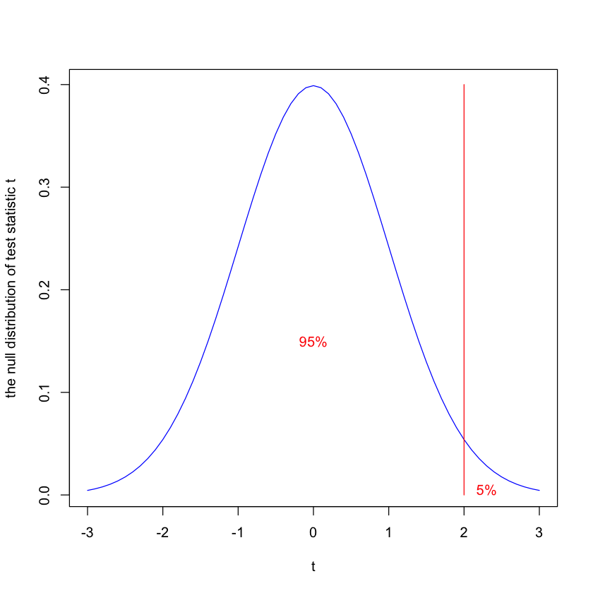
Rejection region: we reject the null if \(t>a\). We find the value of \(a\) by controling type I error at the level of 5%, i.e.,
Thus, \(a\) is the 95% quantile of the null distribution of the test statistic \(t\).
x <- seq(-3, 3, by = .1)
y <- dnorm(x, mean = 0, sd = 1)
plot(x,y,type="l",col="blue",ylab="the null distribution of test statistic t",xlab="t")
lines(c(2,2),c(0,0.4),col="red")
text(2.3,0.005,labels="5%", col="red")
text(0,0.15,labels="95%", col="red")
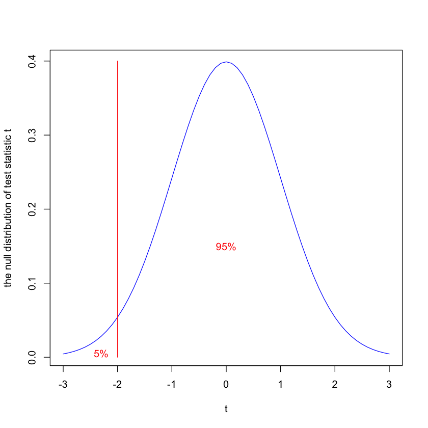
If the alternative is \(H_1\): \(\mu<1\), we only need to change the rejection region and we reject the null if \(t<a\) where \(a\) is the 5% quantile of the null distribution of the test statistic.
x <- seq(-3, 3, by = .1)
y <- dnorm(x, mean = 0, sd = 1)
plot(x,y,type="l",col="blue",ylab="the null distribution of test statistic t",xlab="t")
lines(c(-2,-2),c(0,0.4),col="red")
text(-2.3,0.005,labels="5%", col="red")
text(0,0.15,labels="95%", col="red")
Here, we use the rejection region to make decisions. Alternatively, we may calculate the pvalue and reject the null if \(\text{pvalue}\le 0.05\). The pvalue is an estimate of the Type I error, defined as
where the critical value \(a\) in the rejection region is replaced by the test statistic calculated from data.
data = rnorm(20, mean=2, sd = 1)
t.test(data, mu = 3, alternative="less")
	One Sample t-test

data:  data
t = -5.0692, df = 19, p-value = 3.407e-05
alternative hypothesis: true mean is less than 3
95 percent confidence interval:
     -Inf 2.284231
sample estimates:
mean of x
 1.913682
Two-sided t-test#
Test-stat: \(t=\frac{\bar{x}-1} {sd(\bar{x})}\). The null distribution of \(t\) is the student \(t\) distribution with degrees of freedom \((n-1)\).
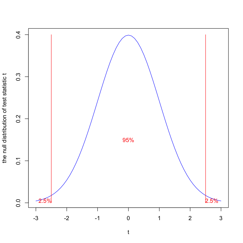
Rejection region: we reject the null if \(t>a\) or \(t<b\), where \(a\) is the 97.5% quantile and \(b\) is the 2.5% quantile of the null distribution of the test statistic.
x <- seq(-3, 3, by = .1)
y <- dnorm(x, mean = 0, sd = 1)
plot(x,y,type="l",col="blue",ylab="the null distribution of test statistic t",xlab="t")
lines(c(2.5,2.5),c(0,0.4),col="red")
lines(c(-2.5,-2.5),c(0,0.4),col="red")
text(2.7,0.005,labels="2.5%", col="red")
text(-2.7,0.005,labels="2.5%", col="red")
text(0,0.15,labels="95%", col="red")
data = rnorm(20, mean=2, sd = 1)
t.test(data, mu = 3, alternative="two.sided")
	One Sample t-test

data:  data
t = -4.2848, df = 19, p-value = 4e-04
alternative hypothesis: true mean is not equal to 3
95 percent confidence interval:
 1.619345 2.525523
sample estimates:
mean of x
 2.072434
Two sample t-test#
Assumption
The two-sample t-test is used to determine if two population means \(\mu_1\) and \(\mu_2\) are equal. The test assumes that the two samples follow the normal distributions, i.e.,
One-sided test#
The test is one-sided if the alternative hypothesis is one-sided.
Test-stat: \(t= \frac{\bar{X_{1}} - \bar{X_{2}}}{\sqrt{{s^{2}_{1}}/n_{1} + {s^{2}_{2}}/n_{2}}}\), where \(n_1\) and \(n_2\) are the sample sizes, \(\bar{X}_1\) and \(\bar{X}_2\) are the sample means, and \(s^2_1\) and \(s_2^2\) are the sample variances.
Rejection region: we reject the null if the test statistic is too large, i.e., \(t>a\) where the critical value \(a\) is the 95% quantile of the t distribution with \(n_1+n_2-2\) degrees of freedom.
Test-stat: the same
Rejection region: we reject the null if the test statistic is \(t<a\) where the critical value \(a\) is the 5% quantile of the t distribution with \(n_1+n_2-2\) degrees of freedom.
group1 = rnorm(20, mean=2, sd = 1)
group2 = rnorm(20, mean=3, sd = 1)
boxplot(cbind(group1,group2))
t.test(group1, group2, alternative="greater")
	Welch Two Sample t-test

data:  group1 and group2
t = -3.8401, df = 34.332, p-value = 0.9997
alternative hypothesis: true difference in means is greater than 0
95 percent confidence interval:
 -1.475106       Inf
sample estimates:
mean of x mean of y
 1.681810  2.706036

Two-sided test#
Test-stat: the same
Rejection region: we reject the null if the test statistic is \(t<a\) or \(t>b\) where the critical values \(a\) and \(b\) are the 97.5% and 2.5% quantile of the t distribution with \(n_1+n_2-2\) degrees of freedom.
t.test(group1, group2, alternative="two.sided")
	Welch Two Sample t-test

data:  group1 and group2
t = -3.8401, df = 34.332, p-value = 0.0005053
alternative hypothesis: true difference in means is not equal to 0
95 percent confidence interval:
 -1.5660716 -0.4823795
sample estimates:
mean of x mean of y
 1.681810  2.706036
F-test for more than two samples#
Assumption
The F-test (ANOVA) can determine whether multiple population means \(\mu_1,\dots,\mu_k\) are equal. The test assumes that the samples follow the normal distributions, i.e.,
…
Test-stat: \(t\) = variation between sample means / variation within the samples
Rejection region: We reject the null if \(t>a\) where \(a\) is the 95% quantile of the F distribution.
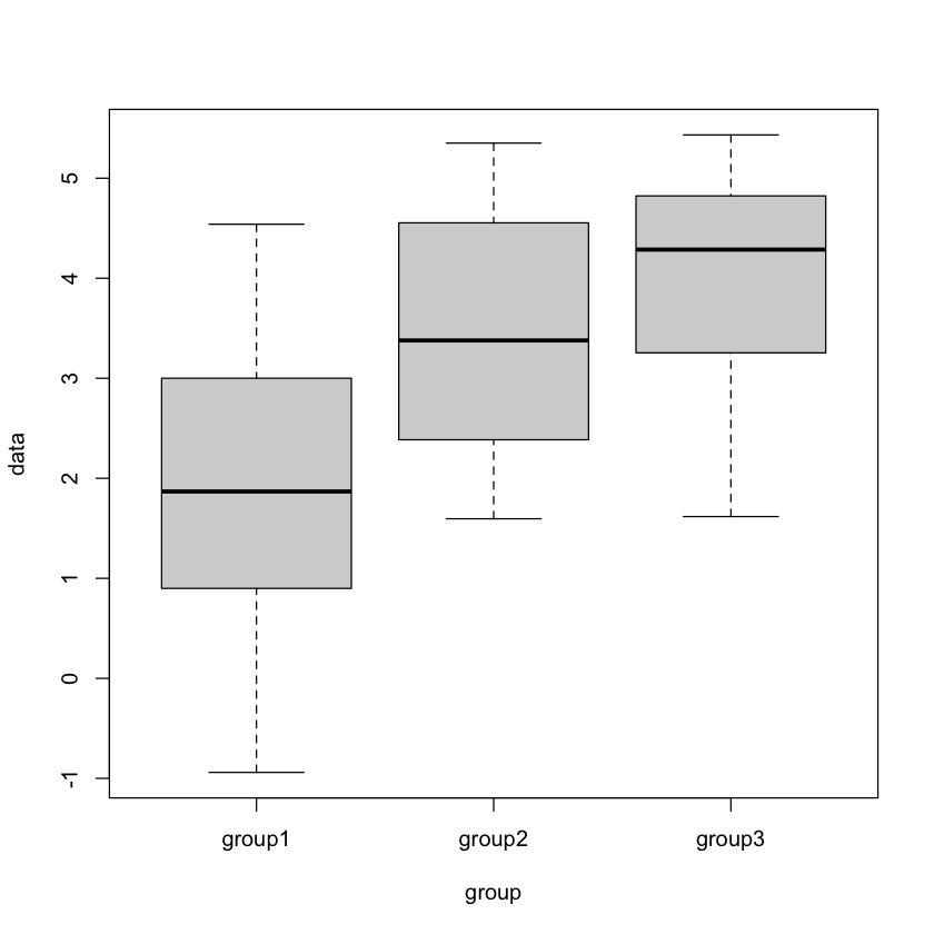
group1 = rnorm(20, mean=2, sd = 1)
group2 = rnorm(20, mean=3.2, sd = 1)
group3 = rnorm(20, mean=4, sd = 1)
data = c(group1,group2,group3)
group= c(rep("group1",20),rep("group2",20),rep("group3",20))
boxplot(data~group)
result = aov(data~group)
summary(result)
            Df Sum Sq Mean Sq F value  Pr(>F)
group        2  44.66  22.332   15.74 3.6e-06 ***
Residuals   57  80.86   1.419
---
Signif. codes:  0 ‘***’ 0.001 ‘**’ 0.01 ‘*’ 0.05 ‘.’ 0.1 ‘ ’ 1
Association test (contingency table):#
Assumption
The association test can determine whether there is association between two variables, for instance, smoking and gender. The test assumes that the counts follow the Poisson distribution.
We randomly take 20 people (12 female and 8 male) and count the number of people who smoke. We want to know if smoking is associated with gender.
\(H_0\) : gender and smoking are independent versus \(H_1\) : not independent
If the null hypothesis is true, then \(P(M\cap S)=P(M) * P(S)=8 / 20 * 9 / 20\). Thus, under the null hypothesis, the expected number of male who smoke is \(8 / 20 * 9 / 20 * 20=3.6\). Similarly, the expected number of female who smoke is \(12 / 20 * 9 / 20 * 20=5.4\). The expected number of male who do not smoke is \(8 / 20 * 11 / 20 * 20=4.4\). The expected number of female who do not smoke is \(12 / 20 * 11 / 20 * 20=6.6\).
Test-stat: \(t=\sum_{i=1}^{4} \frac{\left(o_{i}-e_{i}\right)^{2}}{e_{i}}\), where \(o_i's\) are the observed counts and \(e_i's\) are the expected counts in the table.
The null distribution of the test statistic is asymptotically (i.e., sample size is large) the \(\chi^2\) distribution with \((r-1)(c-1)\) degrees of freedom, in which \(r\) is the number of rows and \(c\) is the number of columns.
Rejection region: we reject the null if \(t>a\), where \(a\) is the 95% quantile of the \(\chi^2\) distribution with \((r-1)(c-1)\) degrees of freedom.
x=matrix(c(6,3,2,9),2,2)
contingency_table = as.table(x)
result = chisq.test(contingency_table)
result
print(paste("the expected count is ",result$expected))
Warning message in chisq.test(contingency_table):
“Chi-squared approximation may be incorrect”
	Pearson's Chi-squared test with Yates' continuity correction

data:  contingency_table
X-squared = 3.0387, df = 1, p-value = 0.0813
[1] "the expected count is  3.6" "the expected count is  5.4"
[3] "the expected count is  4.4" "the expected count is  6.6"
Likelihood ratio test#
Assumption
The likelihood ratio test can test which hypothesis (null or alternative) has a better fit to the real data. The test assumes that the likelihood function is given.
Two points hypothesis#
\(H_{0}: \theta=\theta_{0}\) vs \(H_{1}: \theta=\theta_{1}\)
Test-stat: \(t=\frac{l_{0}}{l_{1}}\), or equivalently, \(t=2 \log \left(l_{1}\right)-2 \log \left(l_{0}\right)\), where \(l_{0}\) is the likelihood under the null hypothesis and \(l_{1}\) is the likelihood under the alternative hypothesis.
Rejection region: we reject the null if \(t>a\), where \(a\) is the 95% quantile of the null distribution of the test statistic.
Example 59
Given a random sample \(X_{1}, X_{2}, \ldots, X_{n} \sim \operatorname{Normal}\left(\mu, \sigma^{2}=1\right)\), we want to test if \(\mu=1\) or \(\mu=2\).
We find the likelihood score \(l_0\) for the null hypothesis
and the likelihood score \(l_1\) for the alternative hypothesis
The test statistic is given by
The null distribution of \(t\) is normal with mean \(-n \mu+\frac{3 n}{2}\) and variance \(n \sigma^{2}\).
Rejection region: we reject the null if \(t>a\), where \(a\) is the 95% quantile of the null distribution of the test statistic \(t\).
x = rnorm(20,mean=2,sd=1)
loglike0 = sum(log(dnorm(x,mean=2,sd=1)))
loglike1 = sum(log(dnorm(x,mean=3,sd=1)))
t = 2*loglike1 - 2*loglike0
a = qchisq(0.95,df=1)
print(paste("the test statistic is",t, "and the critical value a =",a))
[1] "the test statistic is -25.9000033079571 and the critical value a = 3.84145882069412"
Lemma 1 (Neyman-Pearson lemma)
The likelihood ratio test for two simple hypotheses is the most powerful test.
Interval hypotheses#
\(H_{0}: \theta \in \Theta_{0}\) vs \(H_{1}: \theta \in \Theta_{1}\)
Test-stat: \(t=2 \log \left(l_{1}\right)-2 \log \left(l_{0}\right)\), where \(l_{0}=\max _{\theta \in \Theta_{0}}\{l(\theta)\}\) is the maximum likelihood score under the null hypothesis and \(l_{1}\) is the maximum likelihood score \(l_{1}=\) \(\max _{\theta \in \Theta_{1}}\{l(\theta)\}\) under the alternative hypothesis.
Rejection region: we reject the null if \(t>a\) where \(a\) is the 95% quantile of the null distribution of the test statistic.
Nested hypotheses#
\(H_{0}: M_{0}\) vs \(H_{1}: M_{1}\) where the null model \(M_0\) is a special case (nested) of the alternative model \(M_1\).
Test-stat: \(t=2 \log \left(l_{1}\right)-2 \log \left(l_{0}\right)\), where \(l_{0}=\max _{\theta \in \mathrm{M}_{0}}\{l(\theta)\}\) is the maximum likelihood score under the null hypothesis and \(l_{1}\) is the maximum likelihood score \(l_{1}=\) \(\max _{\theta \in \mathrm{M}_{1}}\{l(\theta)\}\) under the alternative hypothesis.
The null distribution of the test statistic is asymptotically the \(\chi^2\) distribution with \(\mathrm{df}=\left(\right.\) number of free parameters in \(H_{1}-\) number of free parameters in \(\left.H_{0}\right)\)
Rejection region: we reject the null if \(t>a\) where \(a\) is the 95% quantile of the chi-square distribution
x = rnorm(20,mean=2,sd=1)
loglike0 = sum(log(dnorm(x,mean=1.2,sd=1)))
loglike1 = sum(log(dnorm(x,mean=mean(x),sd=1)))
t = 2*loglike1 - 2*loglike0
a = qchisq(0.95,df=1)
print(paste("the test statistic is",t, "and the critical value a =",a))
[1] "the test statistic is 4.36725719895644 and the critical value a = 3.84145882069412"
Mann-Whitney test (nonparametric test for two samples)#
Assumption
The Mann-Whitney test can test if two populations have the same median. The test does not assume any underlying probability distribution. This is a nonparametric test.
The data consist of two random samples. Let \(X_{1}, \dots, X_{n}\) be the sample generated from population 1 and \(Y_{1}, \dots, Y_{m}\) be the sample from population 2. We want to test if two samples are from the same population, i.e.,
Test-stat: Ranking all observations from the minimum to the maximum. If several sample values are exactly equal to each other (tied), assign to each the average rank. Let \(\mathrm{R}\left(X_i\right)\) denote the ranks of \(X_i\). The test statistic is \(T=\sum_{i=1}^{n} R\left(X_i\right)\).
Under the null hypothesis that two samples are generated from the same population, the ranks of \(X\) and \(Y\) are totally random. Thus, the ranks of \(X\) (assuming no ties) are \(n\) numbers chosen at random without replacement from \((1,2, \ldots, n+m)\). The null distribution of \(T\) can be derived for small \(\mathrm{n}\) and \(\mathrm{m}\) (table). For large \(n\) and \(m\), we can use simulation to calculate the null distribution of \(T\).
Rejection region: we reject the null hypothesis if \(t>a\) or \(t<b\), where \(a\) is the 97.5% quantile of the null distribution of the test statistic, and \(b\) is the 2.5% quantile of the null distribution of the test statistic.
Example 60
Data is given in the table. The numbers within the parentheses are ranks. For example, the rank of 2.3 is 5 and the rank of 1.4 is 1.
Test-stat: Let \(R_i\) be the sum of the ranks in group \(i\). Define \(U_i=n_1n_2+\frac{n_i(n_i+1)}{2}-R_i\). The test statistic \(t\) is the smaller of \(U_1\) and \(U_2\), i.e., \(t=min(U_1, U_2)\).
Rejection region: we reject the null hypothesis if \(t>a\) or \(t<b\), where \(a\) is the 97.5% quantile of the null distribution of the test statistic, and \(b\) is the 2.5% quantile of the null distribution of the test statistic.
x=c(2.3,1.4,1.6,1.8)
y=c(1.5,3.7,3.2,2.8,3.3)
wilcox.test(x,y)
	Wilcoxon rank sum exact test

data:  x and y
W = 3, p-value = 0.1111
alternative hypothesis: true location shift is not equal to 0