Lab 3: The law of large numbers

The law of large numbers states that as the sample size \(n\) goes to infinity the sample average \(\bar{X}\) converges to the true population mean \(\mu\) , i.e., as \(n\rightarrow \infty\) , \(\bar{X}\rightarrow \mu\) . In this lab, we will simulate data to demonstrate the law of large numbers.

A discrete case (Poisson distribution)

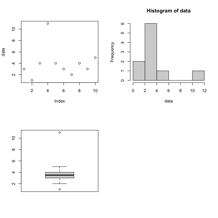
The population mean of the Poisson distribution \((\lambda=5)\) is \(E(X)=\lambda=5\). We simulate \(n=10\) observations from the Poisson distribution and calculate the sample average.

n=10
data = rpois(n, lambda=5)

print(paste("the sample average is",mean(data)))
sd(data)
summary(data)
sort(data)
max(data)
min(data)
quantile(data, prob=0.95)

par(mfrow=c(2,2))
plot(data)
hist(data)
boxplot(data)

[1] "the sample average is 4"

2.70801280154532

   Min. 1st Qu.  Median    Mean 3rd Qu.    Max. 
    1.0     3.0     3.5     4.0     4.0    11.0 

1. 1
2. 2
3. 3
4. 3
5. 3
6. 4
7. 4
8. 4
9. 5
10. 11

11

1

95%: 8.29999999999999

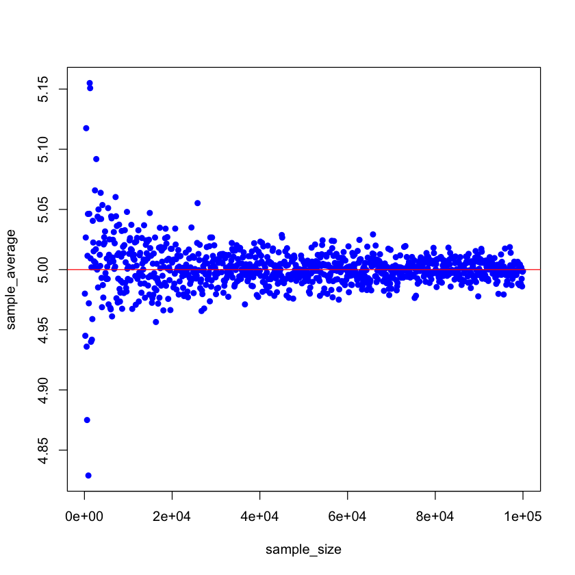
Then we increase the sample size \(n\) from 100, 200, up to 100,000 and recalculate the sample average. By the law of large numbers, we expect that the sample average gets closer to the true population mean 5 as the sample size increases.

nsim = 1000
sample_size = (1:nsim)*100
sample_average = 1:nsim
for(i in 1:nsim){
	data = rpois(sample_size[i],lambda=5)
	sample_average[i] = mean(data)
}

plot(x=sample_size, y=sample_average,col='blue',pch=16)
abline(a=5,b=0,col='red')

A continuous case (Normal distribution)

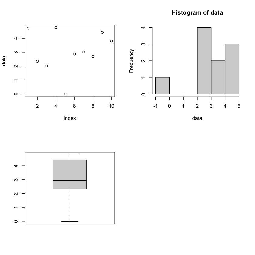
In this case, the population is a normal distribution with mean 2.7 and variance 1.6. We simulate data from \(Normal(\mu=2.7, \sigma^2=1.6)\) and calculate the sample average.

n=10
data = rnorm(n, mean=2.7, sd=sqrt(1.6))

print(paste("the sample average is",mean(data)))
sd(data)
summary(data)
sort(data)
max(data)
min(data)
quantile(data, prob=0.95)

par(mfrow=c(2,2))
plot(data)
hist(data)
boxplot(data)

[1] "the sample average is 3.06171170701605"

1.47026633616873

    Min.  1st Qu.   Median     Mean  3rd Qu.     Max. 
-0.01974  2.42655  2.93877  3.06171  4.27034  4.78223 

1. -0.0197368225213488
2. 2.00174372407675
3. 2.33999065904709
4. 2.6862366733661
5. 2.86452177199222
6. 3.01300876088124
7. 3.79575969152683
8. 4.4285323154812
9. 4.72482636673622
10. 4.78223392957418

4.78223392957418

-0.0197368225213488

95%: 4.7564005262971

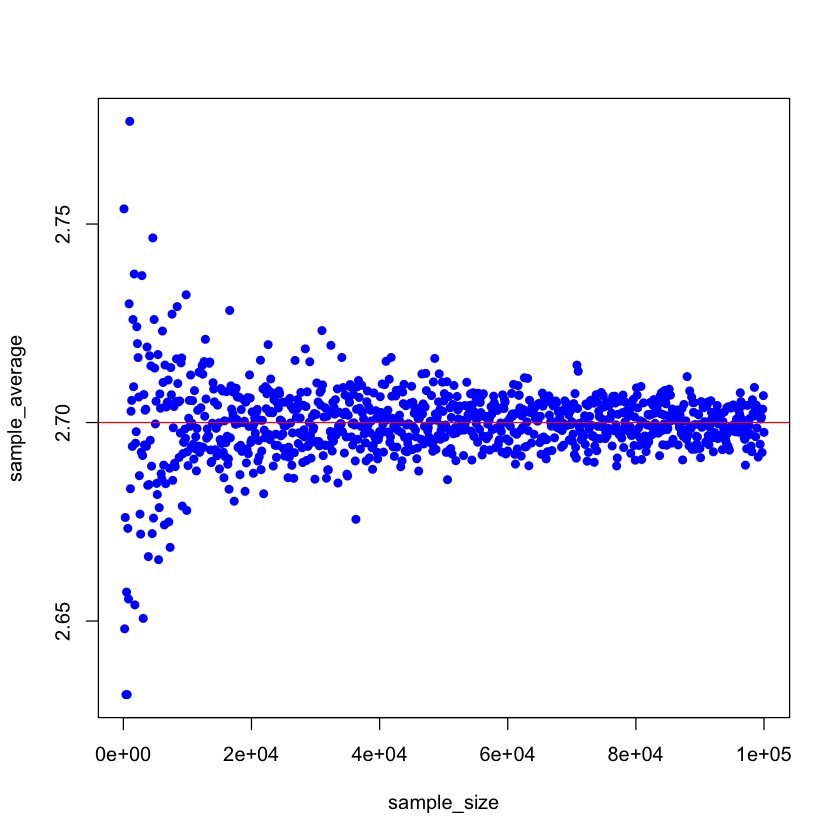
Then we increase the sample size \(n\) from 100, 200, up to 100,000 and recalculate the sample average. By the law of large numbers, we expect that the sample average gets closer to the true population mean 2.7 as the sample size increases.

nsim = 1000
sample_size = (1:nsim)*100
sample_average = 1:nsim
for(i in 1:nsim){
	data = rnorm(sample_size[i],mean=2.7,sd=sqrt(1.6))
	sample_average[i] = mean(data)
}

plot(x=sample_size, y=sample_average,col='blue',pch=16)
abline(a=2.7,b=0,col='red')

Exercise

Demonstrate the law of large numbers for the Binomial distribution, the Exponential distribution, and the Gamma distribution.