Chapter 3: Continuous random variables

“Do the difficult things while they are easy and do the great things while they are small. A journey of a thousand miles must begin with a single step.”

—Lao Tzu

See also

• Continuous probability distribution

Definition 11 (cumulative distribution function)

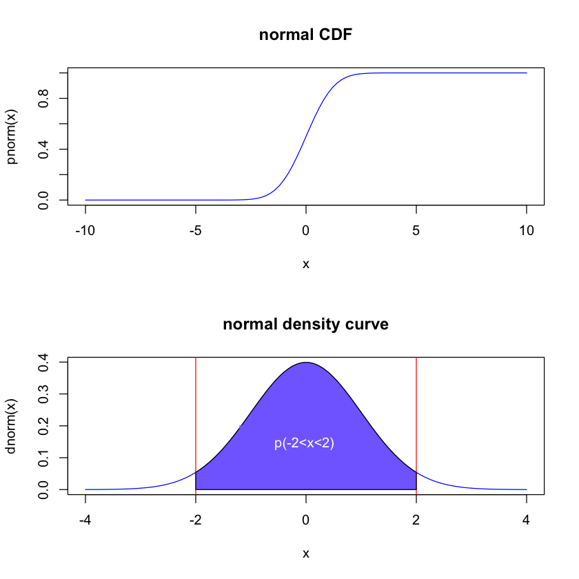
The cumulative distribution function (CDF) of a real-valued random variable \(X\), evaluated at \(x\), is the probability that \(X\) will take a value less than or equal to \(x\), i.e.,

\[F(x)=P(X \leq x)\]

• \(0\le F(x)\le 1\)

• If \(x\le y\), then \(F(x)\le F(y)\). The CDF is a monotone increasing function

• \(\lim_{x\rightarrow -\infty} F(x) = P(X<-\infty) = 0\)

• \(\lim_{x\rightarrow \infty} F(x) = P(X<\infty) = 1\)

Show code cell source Hide code cell source

par(mfrow=c(2,1))
# plot normal CDF
curve(pnorm, from = -10, to = 10,col="blue", main="normal CDF")
# plot normal density
curve(dnorm, from=-4, to=4, col="blue", main="normal density curve")
abline(v=c(-2,2),col="red")

# shade the area under the curve
x = seq(-4,4,by=0.01)
y = dnorm(x)
den <- data.frame(x,y)

value1=-2
value2=2
polygon(c(value1,den$x[den$x >= value1 & den$x <= value2],value2),
        c(0, den$y[den$x >= value1 & den$x <= value2 ],0),
        col = "slateblue1", border = 1)
legend(-1.2,0.2,"p(-2<x<2)", text.col="white", border="slateblue1",fill="slateblue1", bg="slateblue1", box.col="slateblue1")

Definition 12 (probability density function)

The probability density function \(f(x)\) is the derivate of the CDF \(F(x)\) at \(x\), i.e.,

\[f(x)=\frac{d F(x)}{d x}\]

• \(f(x)\ge 0\) because the CDF \(F(x)\) is a monotone increasing function.

• \(F(x)=\int_{-\infty}^{x} f(y) d y\).

• \(\int_{-\infty}^\infty f(x)dx = 1\), i.e., the total probability is 1.

• The probability \(P(a<X<b)\) is the area under the density curve \(f(x)\) between \(a\) and \(b\), i.e.,

\[P(a<X<b) = \int_a^b f(x)dx\]

Definition 13 (expectation)

Let \(f(x)\) be the density function of a continuous random variable \(X\). The expectation of \(X\) is defined as

\[E(X)=\int_{-\infty}^{\infty} x f(x) d x\]

The expectation \(E(X)\) is also called the population mean.

Moreover, the expectation of the function \(g(X)\) is defined as

\[E(g(X))=\int_{-\infty}^{\infty} g(x) f(x) d x\]

The variance of \(X\) is defined as

\[var(X) = E(X-E(X))^2\]

The standard deviation of \(X\) is equal to the square root of the variance, i.e., \(sd(X) = \sqrt{var(X)}\).

Theorem 9

Consider a continuous random variable \(X\) with a probability density function \(f(x)\). Let \(Y = aX + b\) be a transformed random variable, where \(a\) and \(b\) are real numbers. The expectation of \(Y\) can be expressed in terms of the expectation of \(X\), i.e., \(E(aX + b) = aE(X) + b\). Moverover, \(var(aX+b) = a^2var(x)\).

Proof. We first show \(E(aX + b) = aE(X) + b\).

\[\begin{split} \begin{equation} \begin{split} E(aX+b) &= \int_{-\infty}^{\infty}(ax+b)f(x)dx \\ &= \int_{-\infty}^{\infty}axf(x)dx + \int_{-\infty}^{\infty}bf(x)dx\\ &= a\int_{-\infty}^{\infty}xf(x)dx + b\int_{-\infty}^{\infty}f(x)dx\\ &= aE(X)+b \end{split} \end{equation} \end{split}\]

Next, we show \(var(aX+b) = a^2var(x)\).

\[\begin{split} \begin{equation} \begin{split} var(aX+b) &= \int_{-\infty}^{\infty}\left(ax+b-(aE(x)+b)\right)^2f(x)dx \\ &= \int_{-\infty}^{\infty}a^2(x-E(x))^2f(x)dx\\ &= a^2var(X) \end{split} \end{equation} \end{split}\]

Theorem 10

For a continuous random variable \(X\), \(var(X) = E(X^2) - \left(E(X)\right)^2\).

Proof. Suppose \(X\) is a continous random variable with a probability density function \(f(x)\).

\[\begin{split} \begin{equation} \begin{split} var(X) &= \int_{-\infty}^{\infty}\left(x-E(x)\right)^2f(x)dx \\ &= \int_{-\infty}^{\infty}(x^2-2xE(x)+E(x)^2)f(x)dx\\ &= \int_{-\infty}^{\infty}x^2f(x)dx-2E(x)\int_{-\infty}^{\infty}xf(x)dx+E(x)^2\int_{-\infty}^{\infty}f(x)dx\\ &= E(X^2) - \left(E(X)\right)^2 \end{split} \end{equation} \end{split}\]

Important

Theorem 9 and Theorem 10 also hold true for discrete random variables.

Continuous probability distributions

Uniform distribution

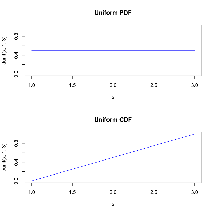
The uniform random variable represents the random numbers in an interval \([a,b]\).

• \(f(x|a,b)=\frac{1}{b-a}\), for \(x \in[a, b]\)

• \(F(x)=P(X \leq x)=\int_{a}^{x} \frac{1}{(b-a)} dy = \frac{x-a}{b-a}\)

• \(E(X)=\int_{a}^{b}xf(x)dx=\int_{a}^{b}\frac{x}{b-a}dx=\frac{a+b}{2}\)

• \(var(X)=E(X^2)-(E(X))^2=\int_{a}^{b}\frac{x^2}{b-a}dx-\big(\frac{a+b}{2}\big)^2=\frac{(b-a)^2}{12}\)

par(mfrow=c(2,1))
curve(dunif(x,1,3), from=1, to=3, main="Uniform PDF", col="blue", ylim=c(0,1))
curve(punif(x,1,3), from=1, to=3, main="Uniform CDF", col="blue", ylim=c(0,1))

Example 25

The random variable \(X\) follows the uniform [2,4]. Find \(E(X)\), \(var(X)\), and \(P(X<2.7)\)

Here, \(a=2\) and \(b=4\). Thus, \(E(X)=(b+a)/2=3\) and \(var(X) = (b-a)^2/12 = 1/3\) and \(P(X<2.7) = (x-a)/(b-a) = 0.7/2=0.35\).

Normal distribution

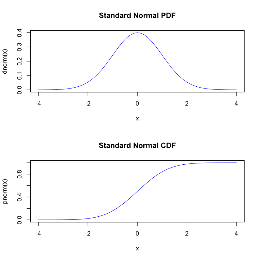
The normal random variable signifies the average outcome of numerous equally probable random variables. For instance, human body weight (or height) is considered a normal random variable as it represents the average effect of multiple factors. The normal distribution is characterized by two parameters: the population mean denoted by \(\mu\) and the population variance denoted by \(\sigma^2\).

• \(f(x|\mu,\sigma^2)=\frac{1}{\sqrt{2 \pi \sigma^{2}}} e^{-\frac{(x-u)^{2}}{2 \sigma^{2}}}\), for \(x \in[-\infty, \infty]\)

• \(E(X)=u\) and \(var(X)=\sigma^{2}\)

Important

The normal density is a bell-shaped curve centered around its mean \(\mu\).

par(mfrow=c(2,1))
curve(dnorm(x), from=-4, to=4, main="Standard Normal PDF", col="blue")
curve(pnorm(x), from=-4, to=4, main="Standard Normal CDF", col="blue")

Suppose \(X\) is a normal random variable \(X\) with mean \(\mu\) and variance \(\sigma^2\). Then, a linearly transformed variable \(Y=aX+b\), where \(a\) and \(b\) are real numbers, is also a normal random variable with mean \(a\mu+b\) and variance \(a^2\sigma^2\).

To calculate the normal probabilities, we first standardize the normal random variable \(\frac{X-E(X)}{sd(X)}\) and then use the standard normal distribution to calculate probabilities,

\[P(X<d)=P\left(\frac{X-u}{\sigma}<\frac{d-u}{\sigma}\right) = P\left(Z<\frac{d-u}{\sigma}\right)\]

68-95-99 rule for the standard normal distribution

1. 68% of the population is within 1 standard deviation of the mean.

2. 95% of the population is within 2 standard deviation of the mean.

3. 99% of the population is within 3 standard deviation of the mean.

Example 26

If \(X \sim Normal(\mu=1,\sigma^2=1)\), find \(E(X^2)\) and \(P(X>2)\)

\(E(X^2) = var(X)+(E(X))^2 = 1+1^2 = 2\) and \(P(X>2) = P\left(\frac{X-\mu}{\sigma}>\frac{2-1}{1}\right)= P(Z>1)\) where \(Z \sim Normal(0,1)\). We know from the 68-95-99 rule that \(P(-1<Z<1) \approx 0.68\). Thus, \(P(Z>1) = (1 - 0.68)/2 = 0.16\).

Exponential distribution

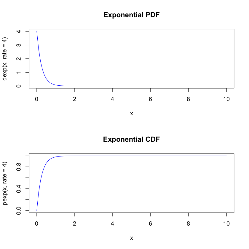
The exponential random variable often represents the waiting time until the next event. For example, the waiting time until the next phone call follows the exponential distribution.

• \(f(x)=\frac{1}{\lambda} e^{-\frac{x}{\lambda}}\), for \(x>0\) and \(\lambda>0\)

• \(F(x)=\int_0^{x}\frac{1}{\lambda} e^{-\frac{y}{\lambda}}dy =1-e^{-\frac{x}{\lambda}}\)

• \(E(X)=\int_0^{\infty}x\frac{1}{\lambda} e^{-\frac{x}{\lambda}}dx=\lambda\)

• \(var(X)=E(X^2)-(E(X))^2=\int_0^{\infty}x^2\frac{1}{\lambda} e^{-\frac{x}{\lambda}}dx-\lambda^2 =\lambda^{2}\)

par(mfrow=c(2,1))
curve(dexp(x,rate=4), 0, 10, main="Exponential PDF",col="blue")
curve(pexp(x,rate=4), 0, 10, main="Exponential CDF",col="blue")

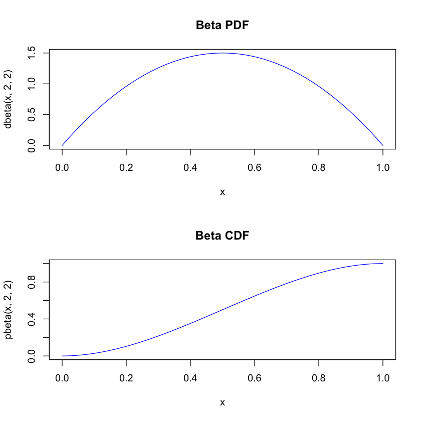
Beta distribution

We often use the Beta distribution to model probabilities because the domain of a Beta random variable is between 0 and 1.

• \(f(x)=\frac{\Gamma(\alpha+\beta)}{\Gamma(\alpha) \Gamma(\beta)} x^{\alpha-1}(1-x)^{\beta-1}, 0 \leq x \leq 1, \alpha>0, \beta>0\)

• \(E(X)=\int_0^1x\frac{\Gamma(\alpha+\beta)}{\Gamma(\alpha) \Gamma(\beta)} x^{\alpha-1}(1-x)^{\beta-1}dx=\frac{\alpha}{\alpha+\beta}\int_0^1\frac{\Gamma(\alpha+1+\beta)}{\Gamma(\alpha+1) \Gamma(\beta)} x^{\alpha+1-1}(1-x)^{\beta-1}dx=\frac{\alpha}{\alpha+\beta}\)

• \(var(X)=E(X^2)-(E(X))^2=\int_0^1x^2\frac{\Gamma(\alpha+\beta)}{\Gamma(\alpha) \Gamma(\beta)} x^{\alpha-1}(1-x)^{\beta-1}-\big(\frac{\alpha}{\alpha+\beta}\big)^2dx=\frac{\alpha \beta}{(\alpha+\beta)^{2}(\alpha+\beta+1)}\)

par(mfrow=c(2,1))
curve(dbeta(x,2,2),0,1, main="Beta PDF",col="blue")
curve(pbeta(x,2,2),0,1, main="Beta CDF",col="blue")

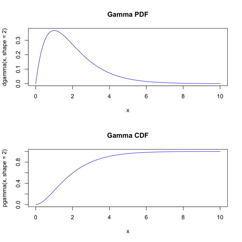
Gamma distribution

We often use the Gamma distribution to model ratios, for example, mutation rates.

• \(f(x)=\frac{1}{\Gamma(\alpha) \beta^{\alpha}} x^{\alpha-1} e^{-\frac{x}{\beta}}, x>0, \alpha>0, \beta>0\)

• \(E(X)=\int_0^{\infty}x\frac{1}{\Gamma(\alpha) \beta^{\alpha}} x^{\alpha-1} e^{-\frac{x}{\beta}}dx=\alpha\beta\int_0^{\infty}\frac{1}{\Gamma(\alpha+1) \beta^{\alpha+1}} x^{\alpha+1-1} e^{-\frac{x}{\beta}}dx =\alpha\beta\)

• \(var(X)=E(X^2)-(E(X))^2=\int_0^{\infty}x^2\frac{1}{\Gamma(\alpha) \beta^{\alpha}} x^{\alpha-1} e^{-\frac{x}{\beta}}dx-(\alpha\beta)^2=(\alpha+1)\alpha\beta^2-\alpha^2\beta^2=\alpha \beta^{2}\)

par(mfrow=c(2,1))
curve(dgamma(x,shape=2), 0, 10, main="Gamma PDF",col="blue")
curve(pgamma(x,shape=2), 0, 10, main="Gamma CDF",col="blue")

Transformation

Three commonly employed techniques can be utilized to determine the probability distribution of a transformed continuous random variable.

CDF

Suppose \(Y=g(X)\) is a transformed random variable, where \(g\) is a bijective function, i.e., its inverse function \(g^{-1}\) exists. We want to find the probability distribution of \(Y\). By definition, the CDF of Y is \(P(Y\le a)\). We apply the inverse function \(g^{-1}\) on both sides of the inequality,

\[ P(Y \le a)=P(g^{-1}(Y)\le g^{-1}(a))=P(X\leq g^{-1}(a))=\int_{-\infty}^{g^{-1}(a)} f(x)dx \]

Example 27

Suppose \(X\) is an exponential random variable with a density \(e^{-x}\). Find the probability distribution of \(Y=2X\)’

\[P(Y\le y) = P(2X \le y) = P(X\le y/2) = 1-e^{-y/2}\]

The density function of \(Y\) is the derivative of the CDF \(1-e^{-y/2}\) with respect to \(y\),

\[(1-e^{-y/2})'=\frac{1}{2}e^{-\frac{y}{2}}\]

This is an exponential density with \(\lambda = 2\).

PDF

Suppose that the inverse function \(g^{-1}(X)\) exists and is an increasing function.

\[ P(Y \leq a)=P(g(X) \leq a)=P\left(X \leq g^{-1}(a)\right)=F_{X}\left(g^{-1}(a)\right) \]

Thus, the density function of \(Y\) is given by

\[ f_{Y}(a)=F^{\prime}{ }_{X}\left(g^{-1}(a)\right)=f_{x}\left(g^{-1}(a)\right) * \frac{d g^{-1}(a)}{d a} \]

If \(g^{-1}(X)\) is a decreasing function, then

\[ P(Y \leq a)=P(g(X) \leq a)=P\left(X > g^{-1}(a)\right)=1-F_{X}\left(g^{-1}(a)\right) \]

and

\[ f_{Y}(a)=-F^{\prime}{ }_{X}\left(g^{-1}(a)\right)=-f_{X}\left(g^{-1}(a)\right) * \frac{d g^{-1}(a)}{d a} \]

Combining two (increasing or decreasing), we have

\[ f_{Y}(y)=f_{X}\left(g^{-1}(y)\right) *\left|\frac{d g^{-1}(y)}{d y}\right| \]

Example 28

The random variable \(X\) is an exponential random variable with density function \(f(x)=\lambda e^{-\lambda x}\). Find the distribution of \(Y=X+2\). The inverse function is \(X=Y-2\). Thus, for \(y>2\)

\[ f_{y}(y)=\lambda e^{-\lambda(y-2)}\left|\frac{d(y-2)}{d y}\right|=\lambda e^{-\lambda(y-2)} \]

MGF (moment generating function)

Let \(M_X(t)\) be the MGF of a random variable \(X\). If two random variables \(X_1\) and \(X_2\) are independent, we can show that the MGF of the sum \(X_1+X_2\) is equal to the product of the MGFs of \(X_1\) and \(X_2\), i.e.,

\[ M_{X_1+X_2}(t)=M_{X_1}(t) M_{X_2}(t) \]

Furthermore, the Moment Generating Function (MGF) of a random variable uniquely determines its probability distribution. Once the MGF is determined, the corresponding probability distribution can be identified.

Example 29

The MGF of a normal random variable is \(e^{u t+\sigma^{2} t^{2} / 2}\). Suppose \(X_{1}, X_{2}, \ldots, X_{n}\) are independent normal random variables with the same mean and variance, i.e., \(Normal\left(u, \sigma^{2}\right)\). Find the probability distribution of the sample average \(\frac{\sum_{i=1}^{n} X_{i}}{n}\).

We first find the MGF of the sum \(\sum_{i=1}^{n} X_{i}\). Because \(X_{1}, X_{2}, \ldots, X_{n}\) are independent random variables, the MGF of the sum \(\sum_{i=1}^{n} X_{i}\) is equal to the product of the MGFs of individual random variables, i.e.,

\[ \prod_{i=1}^{n} M(t)=e^{n u t+n \sigma^{2} t^{2} / 2} \]

This is the MGF of a normal random variable with mean \(n\mu\) and variance \(n\sigma^2\). Hence, the sum \(\sum_{i=1}^{n} X_{i}\) has a normal distribution with mean \(n \mu\) and variance \(n \sigma^{2}\).

Let \(Y=\sum_{i=1}^{n} X_{i}\) and \(Z=\frac{Y}{n}\). Then, the MGF of \(Z\) is given by

\[E\left(e^{t Z}\right)=E\left(e^{\frac{t Y}{n}}\right)=e^{u t+\frac{\sigma^{2} t^{2}}{2 n}}\]

This is the MGF of a normal random variable with mean \(\mu\) and variance \(\frac{\sigma^{2}}{n}\). Thus, the sample average \(\frac{1}{n}\sum_{i=1}^{n} X_{i}\) has a normal distribution with mean \(\mu\) and variance \(\frac{\sigma^{2}}{n}\).