Lab 10: Monte Carlo simulation

In statistical inference, it is essential to calculate probabilities and expectations. Given a probability density function \(f(x)\), the probability \(P(a<X<b)\) is given by an integral

\[P(a<X<b)=\int_a^bf(x)dx \]

Similarly, the expectation of a function \(g(x)\) is given by

\[E(g(X))=\int_{-\infty}^{\infty}g(x)f(x)dx\]

Both calculations involve integrals with respect to the probability density function \(f(x)\). However, there is often no analytic solution to these integrals. We will use numerical approaches to approximate the integrals.

Monte carlo simulation for integrals

The integral can be approximated by Monte Carlo simulation, where the integral is treated as an expectation \(E(g(X))\) of a function \(g(X)\). By the law of large numbers, the expectation \(E(g(X))\) can be approximated by the sample average \(\overline{g(X)}\). Monte Carlo simulation involves the following steps

Algorithm 4

Input: the target function \(g(x)\) and the density function \(f(x)\)

Output: approximation to the integral

1. Convert the integral to an expectation with respect to a probability density function \(f(x)\), i.e. \(\int_a^b k(x) d x=\int_a^b g(x) f(x) d x=E(g(x))\)

2. Generate a random sample \(x_1, \ldots, x_n\) from the probability distribution \(f(x)\)

3. Calculate the sample average of \(\overline{g(x)}=\frac{g\left(x_1\right)+\cdots+g\left(x_n\right)}{n}\)

Example

Calculate \(\int_0^2 \log (x) e^{2x} dx\)

\[\begin{split} \begin{equation} \begin{split} \int_0^2 \log (x) e^{2x} * \frac{1}{2}*2 dx &=\int_0^2 2 \log (x) e^{2x} * \frac{1}{2} dx \\ &=\int_0^2 2\log (x) e^{2x}*f(x) dx \\ &=E(g(x)) \end{split} \end{equation} \end{split}\]

where \(g(x)=2 \log (x) e^{2 x}\) and \(f(x)=\frac{1}{2}\) is the density function of Uniform(0, 2). Therefore, Monte Carlo simulation involves the following steps

1. generate a random sample \(x_1, \ldots, x_n\) from Uniform \((0,2)\)

2. calculate \(g\left(x_1\right), \ldots, g\left(x_n\right)\)

3. \(\int_0^{2} \log (x) e^{2 x} d x \approx \frac{g\left(x_1\right)+\cdots+g\left(x_n\right)}{n}\)

A large sample size \(n\) indicates more accurate approximation

sample_size = 100
x = runif(sample_size, 0, 2)
gfunction = 2*log(x)*exp(2*x)
g_average = mean(gfunction)
g_average

11.5305593051881

Monte carlo simulation for variance

Monte Carlo simulation can be employed to compute the variance of an arbitrary estimator \(\hat{\theta} = g\left(x_1, \ldots, x_n\right)\), where \(x_1, \ldots, x_n\) represents a random sample generated from a probability distribution \(f(x)\). Given the probability distribution \(f(x)\) and the specified sample size \(n\), the steps for Monte Carlo simulation to calculate \(\operatorname{var}(\hat{\theta})\) include:

Algorithm 5

1. generate multiple random samples from the probability distribution \(f(x)\); each sample contains \(\mathrm{n}\) observations

   sample 1: \(x_1^{(1)}, \ldots, x_n^{(1)}\)
   sample 2: \(x_1^{(2)}, \ldots, x_n^{(2)}\)
   Sample k: \(x_1^{(k)}, \ldots, x_n^{(k)}\)

2. for each sample, we calculate \(\hat{\theta}\)

   sample 1: \(x_1^{(1)}, \ldots, x_n^{(1)}=>\widehat{\theta_1}\)
   sample 2: \(x_1^{(2)}, \ldots, x_n^{(2)}=>\widehat{\theta_2}\)
   Sample k: \(x_1^{(k)}, \ldots, x_n^{(k)}=>\widehat{\theta_k}\)

3. finally, \(\operatorname{var}(\hat{\theta}) \approx\) the sample variance of \(\widehat{\theta_1}, \ldots, \widehat{\theta_k}=\frac{1}{k-1} \sum_{i=1}^k\left(\widehat{\theta_t}-\overline{\hat{\theta}}\right)^2\) where \(\overline{\hat{\theta}}=\) \(\frac{\widehat{\theta_1}+\cdots+\widehat{\theta_k}}{k}\)

As an illustration, we use Monte Carlo simulation to compute the variance of the sample average for data generated from the exponential distribution.

sample_size = 10
k = 1000
statistic = 1:k
for(i in 1:k){
	sample = rexp(sample_size, rate=1/5)
	statistic[i] = mean(sample)
}
var(statistic)

2.38588795009839

Monte carlo simulation for the null distribution of a test statistic

Monte Carlo simulation can be employed to approximate the null distribution of an arbitrary test statistic \(t\). Suppose \(f(x)\) is the density function of the null model. If \(f(x)\) includes unknown parameters, these parameters are substituted with their estimates, such as maximum likelihood estimates, to generate random samples from the null model \(f(x)\). The steps for Monte Carlo Simulation to approximate the null distribution of an arbitrary test statistic \(t\) include:

Algorithm 6

Input: the test statistic and the null hypothesis

Output: the null distribution of the test statistic

1. generate multiple random samples from the probability distribution \(f(x)\); each sample contains \(n\) observations

   sample \(1: x_1^{(1)}, \ldots, x_n^{(1)}\)
   sample \(2: x_1^{(2)}, \ldots, x_n^{(2)}\)
   ….
   sample k: \(x_1^{(k)}, \ldots, x_n^{(k)}\)

2. for each sample, we calculate \(t\)

   sample \(1: x_1^{(1)}, \ldots, x_n^{(1)}=>t_1\)
   sample \(2: x_1^{(2)}, \ldots, x_n^{(2)}=>t_2\)
   Sample k: \(x_1^{(k)}, \ldots, x_n^{(k)}=>t_k\)

3. The null distribution of \(t\) is approximated by \(t_1, \ldots, t_k\). For example, the \(95 \%\) quantile of the null distribution of \(t\) is approximately equal to the \(95 \%\) quantile of \(t_1, \ldots, t_k\).

Data are generated from the exponential distribution with \(\lambda = 5\).

data = rexp(20, rate = 0.2)
t = mean(data)

We want to test if the population mean \(\lambda\) is equal to 3.

\(H_0: \lambda = 3\) and \(H_1: \lambda > 3\)

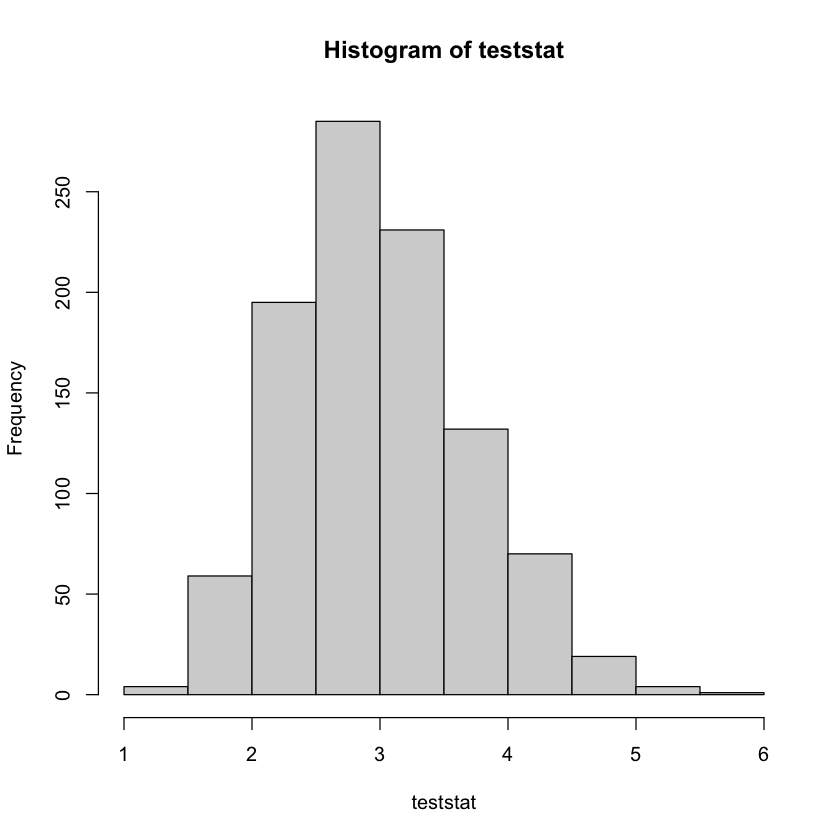
The test statistic is the sample average \(\bar{x}\). We use MC simulation to find the null distribution of the test statistic. The pvalue is equal to the proportion of simulated samples whose sample averages are greater than the sample average \(t\) of data.

sample_size = 20
lambda = 3
k = 1000
teststat = 1:k
for(i in 1:k){
	sample = rexp(sample_size, rate=1/lambda)
	teststat[i] = mean(sample)
}

hist(teststat)

pvalue = sum(teststat>t)/length(teststat)
print(paste("pvalue =", pvalue))

[1] "pvalue = 0.265"