Chapter 2: Discrete random variables

“Do the difficult things while they are easy and do the great things while they are small. A journey of a thousand miles must begin with a single step.”

—Lao Tzu

See also

• Discrete probability distribution

Random variables

Definition 3 (random variable)

A random variable \(X: \Omega\rightarrow E\) is a measurable function from a set \(\Omega\) of outcomes to some set \(E\) of numbers.

1. A random variable is a mapping from outcomes to numbers

2. A random variable can take on different values, each with a probability.

The probability distribution of a random variable \(X\) is a list of all possible values of \(X\) and corresponding probabilities.

Example 8

In an experiment of flipping a fair coin, there are two possible outcomes - head or tail. Define a random variable \(X=0\) for head and \(X=1\) for tail. Then, \(P(X=0)=P(head)=0.5\) and \(P(X=1)=P(tail)=0.5\). The probability distribution of \(X\) is represented by the following table.

\(x\)	0	1
\(p\)	0.5	0.5

Discrete random variables

The possible values of a discrete random variable \(X\) are countable (often integers). Each value of \(X\) has a probability measure \(0 \leq p \leq 1\), and the total probability must be 1.

Definition 4 (probability mass function)

The probability mass function (PMF) of a discrete random variable \(X\) is defined as \(P(X=a)\).

For a function to be a Probability Mass Function (PMF), it must adhere to two conditions: (1) the probability value \(P(X=a)\) must fall within the range of 0 to 1, and (2) the cumulative probability across all possible outcomes must sum to 1.

Example 9

Show that the following table is a probablity mass function.

\(x\)	0	1
\(p\)	0.5	0.5

We verify two conditions: (1) the values of \(p\) are 0.5, falling within the range of 0 to 1, and (2) the total probability sums up to \(0.5+0.5=1\). Therefore, it satisfies the criteria to be a Probability Mass Function (PMF).

Definition 5 (cumulative distribution function)

The cumulative distribution function (CDF) of a discrete random variable \(X\) is defined as \(P(X \leq a)\) for \(a\in \mathbb{R}\).

Example 10

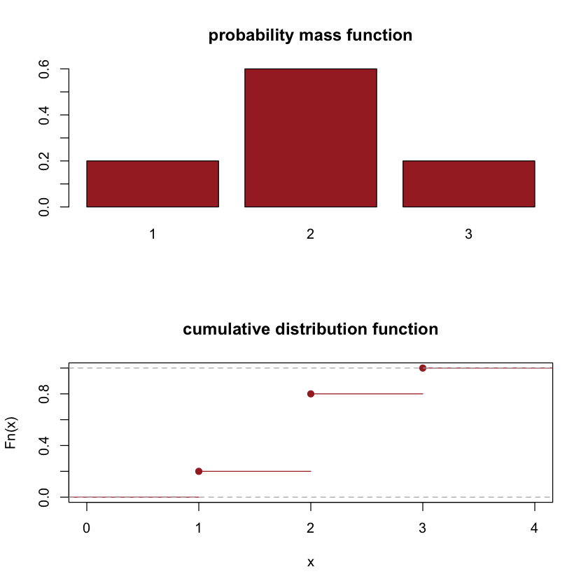
The probability mass function of a discrete random variable \(X\) is given in the following table.

\(x\)	1	2	3
\(p(x)\)	0.2	0.6	0.2

The cumulative probability function is given by

\[\begin{split} F(a)=\begin{equation} \begin{cases} 0 & \text { if } a<1 \\ 0.2 & \text { if } 1 \leq a<2 \\ 0.8 & \text { if } 2 \leq a<3 \\ 1 & \text { if } a \geq 3 \end{cases} \end{equation} \end{split}\]

par(mfrow=c(2,1))
barplot(c("1"=0.2,"2"=0.6,"3"=0.2),col="brown",main="probability mass function")
plot(ecdf(c(rep(1,2),rep(2,6),rep(3,2))),col="brown",main="cumulative distribution function")

Expectations

Definition 6 (expectation)

For a discrete random variable \(X\), the expectation of a function \(g(X)\) of \(X\) is defined as

\[E(g(X))=\sum_{x} g(x) P(x)\]

Example 11

The probability mass function of a discrete random variable \(X\) is given in the following table.

\(x\)	1	2	3
\(p(x)\)	0.2	0.6	0.2

\(E(\log (X))=\sum_{x} \log (x) P(x)=\log (1) * 0.2+\log (2) * 0.6+\log (3) * 0.2=0.6356\)

x = 1:3
p = c(0.2,0.6,0.2)
result=sum(log(x)*p)
print(paste("the expectation is",result))

[1] "the expectation is 0.635610766069589"

Definition 7 (mean)

For a discrete random variable \(X\), the mean of \(X\) is defined as

\[E(X)=\sum_{x} x P(x)\]

Example 12

The probability mass function of a discrete random variable \(X\) is given in the following table.

\(x\)	1	2	3
\(p(x)\)	0.2	0.6	0.2

\(E(X)=\sum_{x} x P(x)=1 * 0.2+2 * 0.6+3 * 0.2=2\)

x = 1:3
p = c(0.2,0.6,0.2)
result = sum(x*p)
print(paste("the mean is",result))

[1] "the mean is 2"

The mean \(E(X)\) of a random variable \(X\) represents the center of a population. The variance of the random variable \(X\) is defined as the average squared distance between each point and the center of a population. The variance represents the spread of a population.

Definition 8 (variance)

For a discrete random variable \(X\), the variance of \(X\) is defined as

\[\operatorname{var}(X)=E\left\{(X-E(X))^{2}\right\}=\sum_{x}(x-E(X))^{2} P(x)\]

The standard deviation (SD) of \(X\) equals the square root of variance, i.e., \(sd(X) = \sqrt{var(X)}\)

Example 13

The probability mass function of a discrete random variable \(X\) is given in the following table.

\(x\)	1	2	3
\(p(x)\)	0.2	0.6	0.2

We find the mean \(E(X)=2\). Thus, \(\operatorname{var}(X)=(1-2)^{2} * 0.2+(2-2)^{2} * 0.6+(3-2)^{2} * 0.2=0.4\)

x = 1:3
p = c(0.2,0.6,0.2)
average = sum(x*p)
variance = sum((x-average)^2*p)
print(paste("variance is",variance))

[1] "variance is 0.4"

Theorem 3

1. \(E(a X+b)=a E(X)+b\)

2. \(\operatorname{var}(a X+b)=a^{2} var(X)\)

3. \(\operatorname{var}(X)=E\left(X^{2}\right)-(E(X))^{2}\)

Proof:

\[\begin{split} \begin{equation} \begin{split} E(aX+b) &= \sum_x(ax+b)P(x) \\ &= \sum_xaxP(x)+\sum_xbP(x) \\ &= a\sum_xxP(x)+b\sum_xP(x) \\ &= aE(X)+b \end{split} \end{equation} \end{split}\]

\[\begin{split} \begin{equation} \begin{split} var(aX+b) &= E[(ax+b-(aE(x)+b))^2]\\ & = E[a^2(x-E(x))^2]\\ & = a^2E[(x-E(x))^2]\\ & = a^2var(X) \end{split} \end{equation} \end{split}\]

\[\begin{split} \begin{equation} \begin{split} var(X) &= E[(x-E(x))^2] \\ &= E(x^2-2xE(x)+(E(x))^2)\\ &=E(x^2)-2E(x)E(x)+(E(x))^2\\ &=E\left(X^{2}\right)-(E(X))^{2} \end{split} \end{equation} \end{split}\]

Example 14

\(x\)	1	2	3
\(p(x)\)	0.2	0.6	0.2

Let \(Y = 3X+6\). Find \(E(Y)\), \(var(Y)\), and \(E(Y^2)\)

We know that \(E(X) = 2\) and \(var(X) = 0.4\). Thus,

\[E(Y)=E(3X+6)=3E(X)+6 = 12\]

and

\[var(Y)=var(3X+6)=9var(X) = 3.6\]

and

\[E(Y^2)=var(Y)+\left(E(X)\right)^2=3.6+144=147.6\]

Definition 9 (moment generating function)

For a discrete random variable \(X\), the moment generating function of \(X\) is defined as

\[E\left(e^{t X}\right)=\sum_{x} e^{t x} P(x)\]

Example 15

\(x\)	1	2	3
\(p(x)\)	0.2	0.6	0.2

The moment generating function is \(M(t) = E\left(e^{t X}\right)= \sum_xe^{tx}p(x)=0.2 e^{t}+0.6 e^{2 t}+0.2 e^{3 t}\)

Theorem 4

For a discrete random variable \(X\), the expectation \(E(X)\) is equal to the derivative of the moment generating function \(M(t)=E(e^{tx})\) evaluated at \(t=0\), i.e.,

\[E(X) = \frac{\partial M(t)}{\partial t}|_{t=0}\]

Proof. The derivative of \(M(t)\) with respect to \(t\) is equal to

\[\begin{split} \begin{equation} \begin{split} \frac{\partial M(t)}{\partial t} &= \frac{\partial \sum_{x} e^{t x} P(x)}{\partial t} \\ &= \sum_{x} \frac{\partial e^{t x} }{\partial t}P(x) \\ &= \sum_{x} xe^{t x}P(x) \end{split} \end{equation} \end{split}\]

When \(t=0\), \(\sum_{x} xe^{t x}P(x) = \sum_{x} xP(x) = E(X)\). Thus, \(E(X) = \frac{\partial M(t)}{\partial t}|_{t=0}\).

Theorem 4 states that we can determine the expected value \(E(X)\) by utilizing the moment generating function \(M(t)\). The expectation \(E(X)\) is alternatively referred to as the first moment. Furthermore, the \(r^{th}\) moment in a discrete probability distribution is defined as \(E\left(X^{r}\right)=\sum_{x} x^{r} P(x)\). It is demonstrated that the \(r^{th}\) moment can be derived from the moment generating function, i.e.,

\[E(X^r)=\frac{\partial^r M(t)}{\partial t^r}|_{t=0}\]

Example 16

\(x\)	1	2	3
\(p(x)\)	0.2	0.6	0.2

Please find \(E(X)\).

From Theorem 4, we can find the expecation using the moment generating function.

\[\begin{split} \begin{equation} \begin{split} E(X) &= \frac{\partial M(t)}{\partial t}|_{t=0}\\ & = (0.2 e^{t}+0.6 e^{2 t}+0.2 e^{3 t})'|_{t=0} \\ & = (0.2 e^{t}+0.6*2e^{2 t}+0.2*3e^{3 t})|_{t=0} \\ & = 0.2+1.2+0.6 = 2 \end{split} \end{equation} \end{split}\]

Definition 10 (probability generating function)

For a discrete random variable, the probability generating function (PGF) is defined as

\[E\left(t^{X}\right)=\sum_{x} t^{x} P(x)\]

While the probability generating function is important in the context of stochastic processes,, its applications within this course are limited.

Example 17

Find the probability generating function for the following probability distribution.

\(x\)	1	2	3
\(p(x)\)	0.2	0.6	0.2

The probability generating function is \(E\left(t^{X}\right)=0.2t+0.6t^2+0.2t^3\)

Discrete probability distributions

Bernoulli random variable

The Bernoulli random variable \(X\) denotes a random event with only two possible outcomes. For example, flipping a coin one time, we may have a head or a tail. The outcome of an exam could be a success or a failure. Success is denoted by 1 and failure is denoted by 0.

• The probablity mass function is given by \(P(X=x)=p^{x}(1-p)^{1-x}\), for \(x=0,1\).

• The expectation of \(X\) is \(E(X)=p\) because \(E(X)=\sum_xxp(x)=0p(0)+1p(1)=p(1)=p\).

• The variance is \(\operatorname{var}(X)=p(1-p)\) because \(var(x)=\sum_x(x-E(x))^2p(x)=(0-p)^2(1-p)+(1-p)^2p=p(1-p)\).

par(mfrow=c(2,1))
barplot(c("0"=0.5,"1"=0.5),col="brown",main="Bernoulli probability mass function")
plot(ecdf(c(0,1)),col="brown",main="Bernoulli cumulative distribution function")

Example 18

The proportions of A, C, G, T in a genome are 25%, 25%, 25%, 25%, respectively. We randomly select two nucleotides. Let \(X\) be the count of A. Find the probability distribution of \(X\).

Let \(X_1\) denote the outcome of the first selection and \(X_2\) be the outcome of the second selection. Both \(X_1\) and \(X_2\) are Bernoulli random variables with \(p=0.25\). Let “A=1” and “not A = 0”. Then, \(X = X_1 + X_2\).

To find the probability distribution of \(X\), we first figure out the possible values that \(X\) may take and then find the corresponding probabilities. It is trivial that \(X\) can take on three values: \(0, 1, 2\). Next, we find the corresponding probabilies,

\(P(X=0) = P(X_1=0 \text{ and } X_2=0) = P(X_1=0)P(X_2=0) = 0.75^2=0.5625\)

\[\begin{split} \begin{equation} \begin{split} P(X=1) &= P(X_1=0\text{ and } X_2=1) + P(X_1=1\text{ and } X_2=0) \\ & = P(X_1=0)P(X_2=1) + P(X_1=1)P(X_2=0) \\ & = 0.25*0.75+0.75*0.25=0.375 \end{split} \end{equation} \end{split}\]

\(P(X=2) = P(X_1=1\text{ and } X_2=1) = 0.25^2=0.0625\)

Thus, the probability distribution of \(X\) is given in the table

\(x\)	0	1	2
\(p(x)\)	0.5625	0.375	0.0625

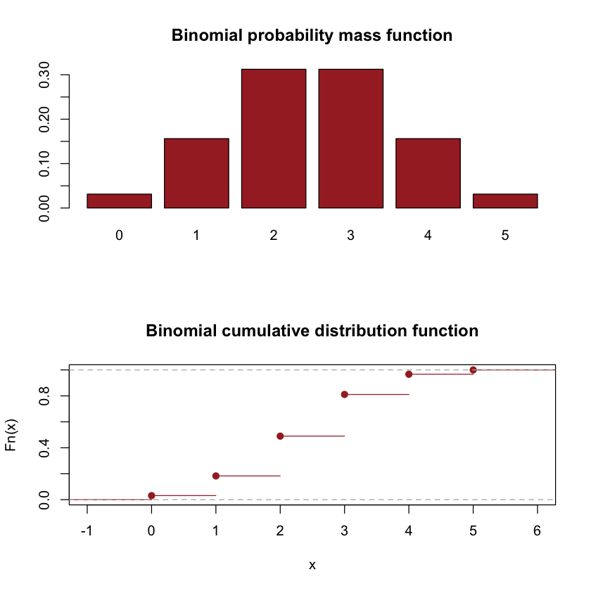
Binomial random variable

The Binomial random variable \(X\) denotes the number of successes in \(n\) trials where each trial may have two possible outcomes - success or failure. For example, the number of heads when flipping a coin \(n\) times. The possible values of \(X\) are \(0, 1, \dots, n\). The probability mass function of the Binomial random variable is for \(x=0,1, \ldots, n\)

\[\begin{split}P(X=x)=\left(\begin{array}{l} n \\x \end{array}\right) p^{x}(1-p)^{n-x}\end{split}\]

Theorem 5

The expectation of the Binomial random variable \(X\) is \(E(X)=np\).

Proof. We find the expectation \(E(X)\) by its definition.

\[\begin{split} \begin{equation} \begin{split} E(X) &= \sum_xxp(x) \\ &= \sum_{x=0}^nx\left(\begin{array}{l} n \\x \end{array}\right) p^{x}(1-p)^{n-x}\\ &=\sum_{x=1}^nx\left(\begin{array}{l} n \\x \end{array}\right) p^{x}(1-p)^{n-x}\\ &=np\sum_{x=1}^{n}x\left(\begin{array}{l} n-1 \\x-1 \end{array}\right) p^{x-1}(1-p)^{(n-1)-(x-1)}\\ &=np\sum_{x=0}^{n-1}x\left(\begin{array}{l} n-1 \\x\end{array}\right) p^{x}(1-p)^{(n-1)-x}\\ &=np \end{split} \end{equation} \end{split}\]

As an exercise, show that the variance is \(\operatorname{var}(X)=np(1-p)\).

par(mfrow=c(2,1))
p = dbinom(0:5,5,0.5)
names(p) = 0:5
barplot(p,col="brown",main="Binomial probability mass function")
plot(ecdf(sample(0:5,size=10000,replace=TRUE, prob=p)),col="brown",main="Binomial cumulative distribution function")

Example 19

The length of a genome is 1 million base pairs with 26% A, 24% C, 25% G, and 25% T. What is the probability that there is a segment in the genome that exactly matches the short read of 5 nucleotides ACCTT? What is the expected number of such segments in the genome?

The probability of the short read is \(P(ACCTT)=P(A)P(C)P(C)P(T)P(T)=0.26*0.24*0.24*0.25*0.25=0.000936\). Let \(X\) be the number of such segments in the genome, which is a Binomial random variable with \(p=0.000936\). Thus, the expected number of ACCTT is \(E(X)=np=10^6*0.000936=936\).

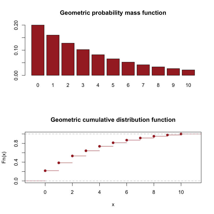
Geometric random variable

The geometric random variable \(X\) denotes the number of failures before observing the first success. The probability mass function of a geometric random variable is for \(x=0,1,2, \ldots\)

\[P(X=x)=p(1-p)^{x}\]

Theorem 6

The expectation of a geometric random variable is \(E(X)=\frac{1-p}{p}\)

Proof. We first find the value of a series \(\sum_{x=0}^{\infty}xt^x\) where \(0<t<1\). Let \(w=\sum_{x=0}^{\infty}xt^x\). Then \(w-wt=\sum_{x=0}^{\infty}t^x=\frac{t}{1-t}\). Thus, \(w=\frac{1}{(1-t)^2}\). Next, we find the expectation \(E(X)\) by its definition.

\[\begin{split} \begin{equation} \begin{split} E(X) &= \sum_xxp(x) \\ &=\sum_{x=0}^{\infty} xp(1-p)^{x}\\ &=p\sum_{x=1}^{\infty} x(1-p)^{x}\\ &=p\frac{1-p}{p^2}=\frac{1-p}{p}\\ \end{split} \end{equation} \end{split}\]

As an exercise, please show that the variance is \(\operatorname{var}(X)=\frac{1-p}{p^{2}}\).

par(mfrow=c(2,1))
p = dgeom(0:10,0.2)
names(p) = 0:10
barplot(p,col="brown",main="Geometric probability mass function")
plot(ecdf(sample(0:10,size=10000,replace=TRUE, prob=p)),col="brown",main="Geometric cumulative distribution function")

Example 20

The length of a genome is 1 million base pairs with 26% A, 24% C, 25% G, and 25% T. We are scanning nucleotides from the left end to the right end of the genome. Let \(X\) be the number of nucleotides until observing the first \(A\). What is the probability \(P(X=2)\)? Find \(E(X)\).

\(X\) is a geometric random variable with the PMF \(p(1-p)^{x}\) where \(p=0.26\). Thus, \(P(X=2)=0.26*(1-0.26)^2=0.142376\). The expectation \(E(X) = \frac{1-p}{p}=\frac{1-0.26}{0.26} = 2.846154\)

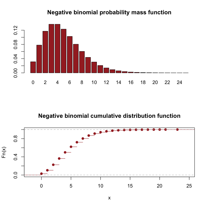
Negative binomial random variable

The negative binomial random variable \(X\) denotes the number of failures before observing the \(r^{th}\) success. Let \(p\) be the probability of a success and \(r\) is the predefined number of successes. The probability mass function of a negative binomial random variable is

\[\begin{split} P(X=x)=\left(\begin{array}{c}x+r-1 \\ x\end{array}\right)p^{r}(1-p)^{x} \end{split}\]

Theorem 7

The expectation of the negative binomial random variable is given by \(E(X)=\frac{r(1-p)}{p}\).

Proof. Let \(X_1\) represent the number of failures until the first success, and \(X_i\) denote the number of failures between the \((i-1)^{th}\) success and the \(i^{th}\) success. It is noteworthy that \(X_i\) follows a Geometric distribution. Consequently, we can express \(X\) as the sum of these variables: \(X=\sum_{i=1}^rX_i\). The expected value of \(X\) can then be computed as

\[E(X)=\sum_{i=1}^rE(X_i)=\sum_{i=1}^r\frac{1-p}{p}=\frac{r(1-p)}{p}\]

Moreover, \(\operatorname{var}(X)=\operatorname{var}(\sum_{i=1}^rX_i)=\frac{r(1-p)}{p^{2}}\).

par(mfrow=c(2,1))
p = dnbinom(0:25,5,0.5)
names(p) = 0:25
barplot(p,col="brown",main="Negative binomial probability mass function")
plot(ecdf(sample(0:25,size=10000,replace=TRUE, prob=p)),col="brown",main="Negative binomial cumulative distribution function")

Example 21

Suppose \(X\) is a negative bionomial random variable with \(p=0.4\) and \(r=2\). Find \(E(X^2)\)

We first find \(E(X) = \frac{r(1-p)}{p} = \frac{2*0.6}{0.4}=3\) and \(var(x)=\frac{r(1-p)}{p^2}=\frac{2*0.6}{0.4^2}=7.5\). Hence, \(E(X^2) = var(X) + (E(X))^2 = 7.5+3^2=16.5\).

Discrete uniform random variable

The discrete uniform random variable is a type of random variable that can take on finitely many values, with each value having an equal probability of occurrence. The probability mass function of the discrete uniform random variable is \(P(X=x)=\frac{1}{n}\) for \(x=a_1,\ldots,a_n\). It is straightforward that the expectation of \(X\) is the average of \(a_1,\dots,a_n\), i.e.,

\[E(X)=\sum_{i=1}^n a_{i} * \frac{1}{n}=\frac{1}{n} \sum_{i=1}^n a_{i}\]

Moreover, \(\operatorname{var}(X)=\sum_{i=1}^n\left(a_{i}-\bar{a}\right)^{2} * \frac{1}{n}\) where \(\bar{a}=\frac{1}{n} \sum_{i=1}^n a_{i}\).

par(mfrow=c(2,1))
p = rep(1/4,4)
names(p) = 1:4
barplot(p,col="brown",main="Discrete uniform probability mass function")
plot(ecdf(1:4),col="brown",main="Discrete uniform cumulative distribution function")

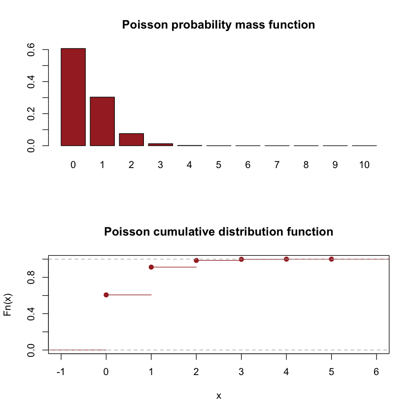
Poisson random variable

The Poisson random variable \(X\) denotes the number of random events during a fixed period of time, for instance, the number of phone calls received between 8am and 8pm, or the number of cars running through a traffic light between October 1 and October 10. The Poisson probability distribution can be obtained from the Poisson process; however, the derivation falls outside the scope of this textbook. The probability distribution of the Poisson random variable is that for \(x=0,1, \ldots\)

\[P(X=x)=\frac{e^{-\lambda}\lambda^{x}}{x!}\]

Note that the total probability is equal to 1, i.e., \(\sum_{x=0}^{\infty}\frac{e^{-\lambda}\lambda^{x}}{x!}=1\).

Theorem 8

The expectation of the Poisson random variable is given by \(E(X)=\lambda\).

Proof. By definition, the expectation of \(X\) is \(E(X)=\sum_xxp(x)\). Thus,

\[\begin{split} \begin{equation} \begin{split} E(X)&=\sum_{x=0}^{\infty}x\frac{e^{-\lambda}\lambda^{x}}{x!}\\ &= \sum_{x=1}^{\infty}x\frac{e^{-\lambda}\lambda^{x}}{x!}\\ &= \lambda \sum_{x=1}^{\infty}\frac{e^{-\lambda}\lambda^{x-1}}{(x-1)!}\\ &= \lambda \sum_{y=0}^{\infty}\frac{e^{-\lambda}\lambda^{y}}{y!}\\ &= \lambda \end{split} \end{equation} \end{split}\]

Moreover, we can show that \(\operatorname{var}(X)=\lambda\). In the case of a Poisson random variable, the expectation is equal to the variance, a defining characteristic of the Poisson probability distribution.

par(mfrow=c(2,1))
p = dpois(0:10, 0.5)
names(p) = 0:10
barplot(p,col="brown",main="Poisson probability mass function")
plot(ecdf(sample(0:10,size=10000,replace=TRUE, prob=p)),col="brown",main="Poisson cumulative distribution function")

Example 22

The length of a genome is 1 million base pairs with 26% A, 24% C, 25% G, and 25% T. Let \(X\) be the number of segments in the genome that exactly matches the short read of 5 nucleotides ACCTT. Find the probability distribution of \(X\).

We have found the probability of a segment ACCTT, \(P(ACCTT)=0.000936\), and \(E(X) = 10^6*0.000936 = 936\). Here, \(X\) is the number of random events (the segment ACCTT) in a genome. Hence, \(X\) is a Poisson random variable with \(\lambda = E(X) = 936\), and the probability distribution is given by \(P(X=x)=\frac{e^{-936}(936)^x}{x!}\) for \(x=0,1,2,\dots\).

Transformation

Most data analysis involves variable transformation. How do we determine the probability distribution of a transformed random variable? We follow two steps: (1) identify all possible values of the transformed variable and (2) find the corresponding probabilities. Let’s explore this through two examples.

Example 23

The probability mass function of a discrete random variable \(X\) is given in the following table.

\(x\)	1	2	3
\(p(x)\)	0.2	0.6	0.2

What is the probability distribution of \(X^2\)? We first identify all possible values of \(X^2\). Since \(X\) can take the values 1, 2, 3, it is straightforward that \(X^2\) can be 1, 4, 9. Next, we find the corresponding probabilities, i.e., \(P(X^2=1) = P(X=1) = 0.2\), \(P(X^2=4) = P(X=2) = 0.6\), \(P(X^2=9) = P(X=3) = 0.2\). Hence, the probability distribution of the transformed random variable \(X^2\) is given by the following table

\(x^2\)	1	4	9
\(p(x^2)\)	0.2	0.6	0.2

Example 24

The probability mass function of a discrete random variable \(X\) is given in the following table

\(x\)	-1	0	1
\(p(x)\)	0.4	0.2	0.4

What is the probability distribution of \(X^2\)? We first identify all possible values of \(X^2\). Since \(X\) can take the values -1, 0, 1, it is straightforward that \(X^2\) can be 0 or 1. Next, we find the corresponding probabilities, i.e., \(P(X^2=0) = P(X=0) = 0.2\), \(P(X^2=1) = P(X=-1)+P(X=1) = 0.8\). Hence, the probability distribution of the transformed random variable \(X^2\) is given by the following table

\(x\)	0	1
\(p(x)\)	0.2	0.8