Lab 8: Linear Discrimination#
Linear Discrimination Analysis#
import numpy as np
from sklearn.datasets import load_iris
from sklearn.discriminant_analysis import LinearDiscriminantAnalysis
from sklearn.model_selection import train_test_split
from sklearn.metrics import accuracy_score

# Load dataset (Iris dataset for example)
data = load_iris()
X = data.data
print(X)
y = data.target

# Split the data into training and testing sets
X_train, X_test, y_train, y_test = train_test_split(X, y, test_size=0.3, random_state=42)

# Create LDA model
lda = LinearDiscriminantAnalysis()

# Fit the model to the training data
lda.fit(X_train, y_train)

# Make predictions on the test data
y_pred = lda.predict(X_test)

# Calculate the accuracy of the model
accuracy = accuracy_score(y_test, y_pred)
print(f"Accuracy: {accuracy:.2f}")

# Optional: print the LDA coefficients
print("LDA Coefficients:")
print(lda.coef_)
[[5.1 3.5 1.4 0.2]
 [4.9 3.  1.4 0.2]
 [4.7 3.2 1.3 0.2]
 [4.6 3.1 1.5 0.2]
 [5.  3.6 1.4 0.2]
 [5.4 3.9 1.7 0.4]
 [4.6 3.4 1.4 0.3]
 [5.  3.4 1.5 0.2]
 [4.4 2.9 1.4 0.2]
 [4.9 3.1 1.5 0.1]
 [5.4 3.7 1.5 0.2]
 [4.8 3.4 1.6 0.2]
 [4.8 3.  1.4 0.1]
 [4.3 3.  1.1 0.1]
 [5.8 4.  1.2 0.2]
 [5.7 4.4 1.5 0.4]
 [5.4 3.9 1.3 0.4]
 [5.1 3.5 1.4 0.3]
 [5.7 3.8 1.7 0.3]
 [5.1 3.8 1.5 0.3]
 [5.4 3.4 1.7 0.2]
 [5.1 3.7 1.5 0.4]
 [4.6 3.6 1.  0.2]
 [5.1 3.3 1.7 0.5]
 [4.8 3.4 1.9 0.2]
 [5.  3.  1.6 0.2]
 [5.  3.4 1.6 0.4]
 [5.2 3.5 1.5 0.2]
 [5.2 3.4 1.4 0.2]
 [4.7 3.2 1.6 0.2]
 [4.8 3.1 1.6 0.2]
 [5.4 3.4 1.5 0.4]
 [5.2 4.1 1.5 0.1]
 [5.5 4.2 1.4 0.2]
 [4.9 3.1 1.5 0.2]
 [5.  3.2 1.2 0.2]
 [5.5 3.5 1.3 0.2]
 [4.9 3.6 1.4 0.1]
 [4.4 3.  1.3 0.2]
 [5.1 3.4 1.5 0.2]
 [5.  3.5 1.3 0.3]
 [4.5 2.3 1.3 0.3]
 [4.4 3.2 1.3 0.2]
 [5.  3.5 1.6 0.6]
 [5.1 3.8 1.9 0.4]
 [4.8 3.  1.4 0.3]
 [5.1 3.8 1.6 0.2]
 [4.6 3.2 1.4 0.2]
 [5.3 3.7 1.5 0.2]
 [5.  3.3 1.4 0.2]
 [7.  3.2 4.7 1.4]
 [6.4 3.2 4.5 1.5]
 [6.9 3.1 4.9 1.5]
 [5.5 2.3 4.  1.3]
 [6.5 2.8 4.6 1.5]
 [5.7 2.8 4.5 1.3]
 [6.3 3.3 4.7 1.6]
 [4.9 2.4 3.3 1. ]
 [6.6 2.9 4.6 1.3]
 [5.2 2.7 3.9 1.4]
 [5.  2.  3.5 1. ]
 [5.9 3.  4.2 1.5]
 [6.  2.2 4.  1. ]
 [6.1 2.9 4.7 1.4]
 [5.6 2.9 3.6 1.3]
 [6.7 3.1 4.4 1.4]
 [5.6 3.  4.5 1.5]
 [5.8 2.7 4.1 1. ]
 [6.2 2.2 4.5 1.5]
 [5.6 2.5 3.9 1.1]
 [5.9 3.2 4.8 1.8]
 [6.1 2.8 4.  1.3]
 [6.3 2.5 4.9 1.5]
 [6.1 2.8 4.7 1.2]
 [6.4 2.9 4.3 1.3]
 [6.6 3.  4.4 1.4]
 [6.8 2.8 4.8 1.4]
 [6.7 3.  5.  1.7]
 [6.  2.9 4.5 1.5]
 [5.7 2.6 3.5 1. ]
 [5.5 2.4 3.8 1.1]
 [5.5 2.4 3.7 1. ]
 [5.8 2.7 3.9 1.2]
 [6.  2.7 5.1 1.6]
 [5.4 3.  4.5 1.5]
 [6.  3.4 4.5 1.6]
 [6.7 3.1 4.7 1.5]
 [6.3 2.3 4.4 1.3]
 [5.6 3.  4.1 1.3]
 [5.5 2.5 4.  1.3]
 [5.5 2.6 4.4 1.2]
 [6.1 3.  4.6 1.4]
 [5.8 2.6 4.  1.2]
 [5.  2.3 3.3 1. ]
 [5.6 2.7 4.2 1.3]
 [5.7 3.  4.2 1.2]
 [5.7 2.9 4.2 1.3]
 [6.2 2.9 4.3 1.3]
 [5.1 2.5 3.  1.1]
 [5.7 2.8 4.1 1.3]
 [6.3 3.3 6.  2.5]
 [5.8 2.7 5.1 1.9]
 [7.1 3.  5.9 2.1]
 [6.3 2.9 5.6 1.8]
 [6.5 3.  5.8 2.2]
 [7.6 3.  6.6 2.1]
 [4.9 2.5 4.5 1.7]
 [7.3 2.9 6.3 1.8]
 [6.7 2.5 5.8 1.8]
 [7.2 3.6 6.1 2.5]
 [6.5 3.2 5.1 2. ]
 [6.4 2.7 5.3 1.9]
 [6.8 3.  5.5 2.1]
 [5.7 2.5 5.  2. ]
 [5.8 2.8 5.1 2.4]
 [6.4 3.2 5.3 2.3]
 [6.5 3.  5.5 1.8]
 [7.7 3.8 6.7 2.2]
 [7.7 2.6 6.9 2.3]
 [6.  2.2 5.  1.5]
 [6.9 3.2 5.7 2.3]
 [5.6 2.8 4.9 2. ]
 [7.7 2.8 6.7 2. ]
 [6.3 2.7 4.9 1.8]
 [6.7 3.3 5.7 2.1]
 [7.2 3.2 6.  1.8]
 [6.2 2.8 4.8 1.8]
 [6.1 3.  4.9 1.8]
 [6.4 2.8 5.6 2.1]
 [7.2 3.  5.8 1.6]
 [7.4 2.8 6.1 1.9]
 [7.9 3.8 6.4 2. ]
 [6.4 2.8 5.6 2.2]
 [6.3 2.8 5.1 1.5]
 [6.1 2.6 5.6 1.4]
 [7.7 3.  6.1 2.3]
 [6.3 3.4 5.6 2.4]
 [6.4 3.1 5.5 1.8]
 [6.  3.  4.8 1.8]
 [6.9 3.1 5.4 2.1]
 [6.7 3.1 5.6 2.4]
 [6.9 3.1 5.1 2.3]
 [5.8 2.7 5.1 1.9]
 [6.8 3.2 5.9 2.3]
 [6.7 3.3 5.7 2.5]
 [6.7 3.  5.2 2.3]
 [6.3 2.5 5.  1.9]
 [6.5 3.  5.2 2. ]
 [6.2 3.4 5.4 2.3]
 [5.9 3.  5.1 1.8]]
Accuracy: 1.00
LDA Coefficients:
[[  6.43431545  16.59042605 -18.91720364 -18.73357838]
 [ -1.22790112  -4.81928389   3.99844288   1.94159565]
 [ -4.16301183  -9.0808028   11.85110611  13.75410516]]
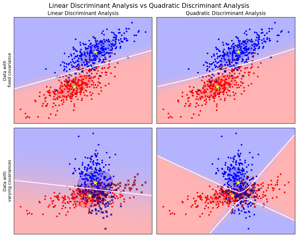
print(__doc__)

from scipy import linalg
import numpy as np
import matplotlib.pyplot as plt
import matplotlib as mpl
from matplotlib import colors

from sklearn.discriminant_analysis import LinearDiscriminantAnalysis
from sklearn.discriminant_analysis import QuadraticDiscriminantAnalysis

#############################################################################
# Colormap
cmap = colors.LinearSegmentedColormap(
    'red_blue_classes',
    {'red': [(0, 1, 1), (1, 0.7, 0.7)],
     'green': [(0, 0.7, 0.7), (1, 0.7, 0.7)],
     'blue': [(0, 0.7, 0.7), (1, 1, 1)]})
plt.cm.register_cmap(cmap=cmap)


#############################################################################
# Generate datasets
def dataset_fixed_cov():
    '''Generate 2 Gaussians samples with the same covariance matrix'''
    n, dim = 300, 2
    np.random.seed(0)
    C = np.array([[0., -0.23], [0.83, .23]])
    X = np.r_[np.dot(np.random.randn(n, dim), C),
              np.dot(np.random.randn(n, dim), C) + np.array([1, 1])]
    y = np.hstack((np.zeros(n), np.ones(n)))
    return X, y


def dataset_cov():
    '''Generate 2 Gaussians samples with different covariance matrices'''
    n, dim = 300, 2
    np.random.seed(0)
    C = np.array([[0., -1.], [2.5, .7]]) * 2.
    X = np.r_[np.dot(np.random.randn(n, dim), C),
              np.dot(np.random.randn(n, dim), C.T) + np.array([1, 4])]
    y = np.hstack((np.zeros(n), np.ones(n)))
    return X, y


#############################################################################
# Plot functions
def plot_data(lda, X, y, y_pred, fig_index):
    splot = plt.subplot(2, 2, fig_index)
    if fig_index == 1:
        plt.title('Linear Discriminant Analysis')
        plt.ylabel('Data with\n fixed covariance')
    elif fig_index == 2:
        plt.title('Quadratic Discriminant Analysis')
    elif fig_index == 3:
        plt.ylabel('Data with\n varying covariances')

    tp = (y == y_pred)  # True Positive
    tp0, tp1 = tp[y == 0], tp[y == 1]
    X0, X1 = X[y == 0], X[y == 1]
    X0_tp, X0_fp = X0[tp0], X0[~tp0]
    X1_tp, X1_fp = X1[tp1], X1[~tp1]

    # class 0: dots
    plt.scatter(X0_tp[:, 0], X0_tp[:, 1], marker='.', color='red')
    plt.scatter(X0_fp[:, 0], X0_fp[:, 1], marker='x',
                s=20, color='#990000')  # dark red

    # class 1: dots
    plt.scatter(X1_tp[:, 0], X1_tp[:, 1], marker='.', color='blue')
    plt.scatter(X1_fp[:, 0], X1_fp[:, 1], marker='x',
                s=20, color='#000099')  # dark blue

    # class 0 and 1 : areas
    nx, ny = 200, 100
    x_min, x_max = plt.xlim()
    y_min, y_max = plt.ylim()
    xx, yy = np.meshgrid(np.linspace(x_min, x_max, nx),
                         np.linspace(y_min, y_max, ny))
    Z = lda.predict_proba(np.c_[xx.ravel(), yy.ravel()])
    Z = Z[:, 1].reshape(xx.shape)
    plt.pcolormesh(xx, yy, Z, cmap='red_blue_classes',
                   norm=colors.Normalize(0., 1.), zorder=0)
    plt.contour(xx, yy, Z, [0.5], linewidths=2., colors='white')

    # means
    plt.plot(lda.means_[0][0], lda.means_[0][1],
             '*', color='yellow', markersize=15, markeredgecolor='grey')
    plt.plot(lda.means_[1][0], lda.means_[1][1],
             '*', color='yellow', markersize=15, markeredgecolor='grey')

    return splot


def plot_ellipse(splot, mean, cov, color):
    v, w = linalg.eigh(cov)
    u = w[0] / linalg.norm(w[0])
    angle = np.arctan(u[1] / u[0])
    angle = 180 * angle / np.pi  # convert to degrees
    # filled Gaussian at 2 standard deviation
    ell = mpl.patches.Ellipse(mean, width=2 * v[0] ** 0.5, height=2 * v[1] ** 0.5, angle=180 + angle, facecolor=color, edgecolor='black', linewidth=2.0)
    ell.set_clip_box(splot.bbox)
    ell.set_alpha(0.2)
    splot.add_artist(ell)
    splot.set_xticks(())
    splot.set_yticks(())


def plot_lda_cov(lda, splot):
    plot_ellipse(splot, lda.means_[0], lda.covariance_, 'red')
    plot_ellipse(splot, lda.means_[1], lda.covariance_, 'blue')


def plot_qda_cov(qda, splot):
    plot_ellipse(splot, qda.means_[0], qda.covariance_[0], 'red')
    plot_ellipse(splot, qda.means_[1], qda.covariance_[1], 'blue')


plt.figure(figsize=(10, 8), facecolor='white')
plt.suptitle('Linear Discriminant Analysis vs Quadratic Discriminant Analysis',
             y=0.98, fontsize=15)
for i, (X, y) in enumerate([dataset_fixed_cov(), dataset_cov()]):
    # Linear Discriminant Analysis
    lda = LinearDiscriminantAnalysis(solver="svd", store_covariance=True)
    y_pred = lda.fit(X, y).predict(X)
    splot = plot_data(lda, X, y, y_pred, fig_index=2 * i + 1)
    plot_lda_cov(lda, splot)
    plt.axis('tight')

    # Quadratic Discriminant Analysis
    qda = QuadraticDiscriminantAnalysis(store_covariance=True)
    y_pred = qda.fit(X, y).predict(X)
    splot = plot_data(qda, X, y, y_pred, fig_index=2 * i + 2)
    plot_qda_cov(qda, splot)
    plt.axis('tight')


plt.tight_layout()
plt.subplots_adjust(top=0.92)
plt.show()
Automatically created module for IPython interactive environment
/var/folders/53/vt_yht0j2h992vrjpc3y4v3cmgg9bt/T/ipykernel_96200/2457434154.py:19: MatplotlibDeprecationWarning: The register_cmap function was deprecated in Matplotlib 3.7 and will be removed two minor releases later. Use ``matplotlib.colormaps.register(name)`` instead.
  plt.cm.register_cmap(cmap=cmap)
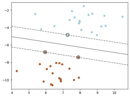
Support Vector Machine#
print(__doc__)

import numpy as np
import matplotlib.pyplot as plt
from sklearn import svm
from sklearn.datasets import make_blobs

# we create 40 separable points
X, y = make_blobs(n_samples=40, centers=2, random_state=6)

# fit the model, don't regularize for illustration purposes
clf = svm.SVC(kernel='linear', C=1000)
clf.fit(X, y)

plt.scatter(X[:, 0], X[:, 1], c=y, s=30, cmap=plt.cm.Paired)

# plot the decision function
ax = plt.gca()
xlim = ax.get_xlim()
ylim = ax.get_ylim()

# create grid to evaluate model
xx = np.linspace(xlim[0], xlim[1], 30)
yy = np.linspace(ylim[0], ylim[1], 30)
YY, XX = np.meshgrid(yy, xx)
xy = np.vstack([XX.ravel(), YY.ravel()]).T
Z = clf.decision_function(xy).reshape(XX.shape)

# plot decision boundary and margins
ax.contour(XX, YY, Z, colors='k', levels=[-1, 0, 1], alpha=0.5,
           linestyles=['--', '-', '--'])
# plot support vectors
ax.scatter(clf.support_vectors_[:, 0], clf.support_vectors_[:, 1], s=100,
           linewidth=1, facecolors='none', edgecolors='k')
plt.show()
Automatically created module for IPython interactive environment