Lab 6: Nonparametric Methods

In nonparametric estimation, we assume that similar inputs have similar outputs. Therefore, the nonparametric algorithm is composed of finding the similar past instances from teh training set using a suitable distance measure and interpolating from them to find the right output.

Nonparametric density estimation

Given the sample \(X\) in the training set, the cumulative distribution function can be estimated by

\[\begin{split}\hat{F}(x) = \frac{\\{x^t \le x\}}{N}\end{split}\]

Let \(h\) be the length of the interval and the instances that fall in this interval are assumed to be close enough. The density can be estimated by

\[\begin{split}\hat{p}(x) = \frac{1}{h}\big{[}\frac{\\{x^t \le x+h\}-\#\{x^t\le x\}}{N}\big{]}\end{split}\]

Histogram estimator

The input space is divided into equal-sized intervals called bins \(\{B_i: i=1,...,k\}\). The histogram estimator for \(p(x)\) is given by

\[\begin{split}\hat{p}(x) = \frac{\\{x^t\in B_x \}}{Nh}\end{split}\]

where \(B_x\) is the bin that \(x\) falls in. In the Naive estimator, the Bin \(B_x\) is replaced by the interval \([x-h/2, x+h/2]\) and the estimator is given by

\[\begin{split}\hat{p}(x) = \frac{\\{-h/2 < x^t < x+h/2\}}{Nh}\end{split}\]

or

\[\hat{p}(x) = \frac{1}{Nh}\sum_{t=1}^Nw\big{(}\frac{x-x^t}{h}\big{)}\]

where \(w\) is the weight function defined as \(w(u) = 1\) if \(|u|<1/2\) and 0 otherwise. Since the weight function is hard (0/1) the estimate is not continuous.

import numpy as np
import matplotlib.pyplot as plt
rng = np.random.RandomState(10)  # deterministic random data
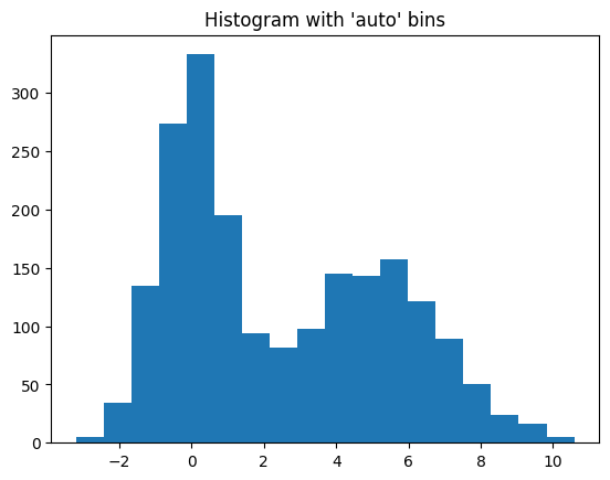
a = np.hstack((rng.normal(size=1000), rng.normal(loc=5, scale=2, size=1000)))
plt.hist(a, bins='auto')  # arguments are passed to np.histogram
plt.title("Histogram with 'auto' bins")
plt.show()

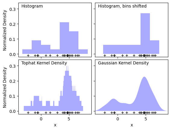
Kernel estimator

The weights in the naive estimator is replaced by a probability distribution \(k(x^t|h,x)\) called kernel. Typically, the kernel is symmetric about \(x\) and truncated by the interval \([x-3h, x+3h]\), i.e.,

\[\hat{p}(x) = \frac{1}{Nh}\sum_{t=1}^Nk\big{(}\frac{x-x^t}{h}\big{)}\]

If \(h\) is small, each training instance has a large effect in a small region and no effect on distant points. When \(h\) is large, there is more overlap of the kernels and we get a smoother estimate.

import numpy as np
import matplotlib
import matplotlib.pyplot as plt
from distutils.version import LooseVersion
from scipy.stats import norm
from sklearn.neighbors import KernelDensity

# `normed` is being deprecated in favor of `density` in histograms
if LooseVersion(matplotlib.__version__) >= '2.1':
    density_param = {'density': True}
else:
    density_param = {'normed': True}

# ----------------------------------------------------------------------
# Plot the progression of histograms to kernels
np.random.seed(1)
N = 20
X = np.concatenate((np.random.normal(0, 1, int(0.3 * N)),
                    np.random.normal(5, 1, int(0.7 * N))))[:, np.newaxis]
X_plot = np.linspace(-5, 10, 1000)[:, np.newaxis]
bins = np.linspace(-5, 10, 10)

fig, ax = plt.subplots(2, 2, sharex=True, sharey=True)
fig.subplots_adjust(hspace=0.05, wspace=0.05)

# histogram 1
ax[0, 0].hist(X[:, 0], bins=bins, fc='#AAAAFF', **density_param)
ax[0, 0].text(-3.5, 0.31, "Histogram")

# histogram 2
ax[0, 1].hist(X[:, 0], bins=bins + 0.75, fc='#AAAAFF', **density_param)
ax[0, 1].text(-3.5, 0.31, "Histogram, bins shifted")

# tophat KDE
kde = KernelDensity(kernel='tophat', bandwidth=0.75).fit(X)
log_dens = kde.score_samples(X_plot)
ax[1, 0].fill(X_plot[:, 0], np.exp(log_dens), fc='#AAAAFF')
ax[1, 0].text(-3.5, 0.31, "Tophat Kernel Density")

# Gaussian KDE
kde = KernelDensity(kernel='gaussian', bandwidth=0.75).fit(X)
log_dens = kde.score_samples(X_plot)
ax[1, 1].fill(X_plot[:, 0], np.exp(log_dens), fc='#AAAAFF')
ax[1, 1].text(-3.5, 0.31, "Gaussian Kernel Density")

for axi in ax.ravel():
    axi.plot(X[:, 0], np.full(X.shape[0], -0.01), '+k')
    axi.set_xlim(-4, 9)
    axi.set_ylim(-0.02, 0.34)

for axi in ax[:, 0]:
    axi.set_ylabel('Normalized Density')

for axi in ax[1, :]:
    axi.set_xlabel('x')

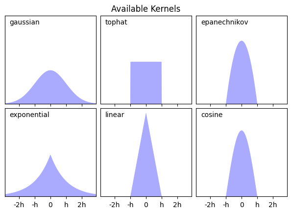
Plot all available kernels

X_plot = np.linspace(-6, 6, 1000)[:, None]
X_src = np.zeros((1, 1))

fig, ax = plt.subplots(2, 3, sharex=True, sharey=True)
fig.subplots_adjust(left=0.05, right=0.95, hspace=0.05, wspace=0.05)


def format_func(x, loc):
    if x == 0:
        return '0'
    elif x == 1:
        return 'h'
    elif x == -1:
        return '-h'
    else:
        return '%ih' % x

for i, kernel in enumerate(['gaussian', 'tophat', 'epanechnikov',
                            'exponential', 'linear', 'cosine']):
    axi = ax.ravel()[i]
    log_dens = KernelDensity(kernel=kernel).fit(X_src).score_samples(X_plot)
    axi.fill(X_plot[:, 0], np.exp(log_dens), '-k', fc='#AAAAFF')
    axi.text(-2.6, 0.95, kernel)

    axi.xaxis.set_major_formatter(plt.FuncFormatter(format_func))
    axi.xaxis.set_major_locator(plt.MultipleLocator(1))
    axi.yaxis.set_major_locator(plt.NullLocator())

    axi.set_ylim(0, 1.05)
    axi.set_xlim(-2.9, 2.9)

ax[0, 1].set_title('Available Kernels')

Text(0.5, 1.0, 'Available Kernels')

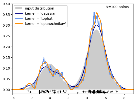
Plot a 1D density

N = 100
np.random.seed(1)
X = np.concatenate((np.random.normal(0, 1, int(0.3 * N)),
                    np.random.normal(5, 1, int(0.7 * N))))[:, np.newaxis]

X_plot = np.linspace(-5, 10, 1000)[:, np.newaxis]

true_dens = (0.3 * norm(0, 1).pdf(X_plot[:, 0])
             + 0.7 * norm(5, 1).pdf(X_plot[:, 0]))

fig, ax = plt.subplots()
ax.fill(X_plot[:, 0], true_dens, fc='black', alpha=0.2,
        label='input distribution')
colors = ['navy', 'cornflowerblue', 'darkorange']
kernels = ['gaussian', 'tophat', 'epanechnikov']
lw = 2

for color, kernel in zip(colors, kernels):
    kde = KernelDensity(kernel=kernel, bandwidth=0.5).fit(X)
    log_dens = kde.score_samples(X_plot)
    ax.plot(X_plot[:, 0], np.exp(log_dens), color=color, lw=lw,
            linestyle='-', label="kernel = '{0}'".format(kernel))

ax.text(6, 0.38, "N={0} points".format(N))

ax.legend(loc='upper left')
ax.plot(X[:, 0], -0.005 - 0.01 * np.random.random(X.shape[0]), '+k')

ax.set_xlim(-4, 9)
ax.set_ylim(-0.02, 0.4)
plt.show()

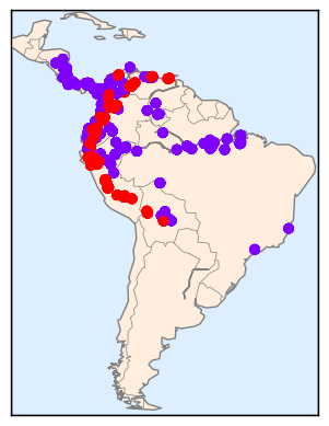
KDE on a sphere

import numpy as np
from sklearn.datasets import fetch_species_distributions

data = fetch_species_distributions()

# Get matrices/arrays of species IDs and locations
latlon = np.vstack([data.train['dd lat'],
                    data.train['dd long']]).T
species = np.array([d.decode('ascii').startswith('micro')
                    for d in data.train['species']], dtype='int')

from mpl_toolkits.basemap import Basemap

def construct_grids(batch):
    """Construct the map grid from the batch object

    Parameters
    ----------
    batch : Batch object
        The object returned by :func:`fetch_species_distributions`

    Returns
    -------
    (xgrid, ygrid) : 1-D arrays
        The grid corresponding to the values in batch.coverages
    """
    # x,y coordinates for corner cells
    xmin = batch.x_left_lower_corner + batch.grid_size
    xmax = xmin + (batch.Nx * batch.grid_size)
    ymin = batch.y_left_lower_corner + batch.grid_size
    ymax = ymin + (batch.Ny * batch.grid_size)

    # x coordinates of the grid cells
    xgrid = np.arange(xmin, xmax, batch.grid_size)
    # y coordinates of the grid cells
    ygrid = np.arange(ymin, ymax, batch.grid_size)

    return (xgrid, ygrid)

xgrid, ygrid = construct_grids(data)

# plot coastlines with basemap
m = Basemap(projection='cyl', resolution='c',
            llcrnrlat=ygrid.min(), urcrnrlat=ygrid.max(),
            llcrnrlon=xgrid.min(), urcrnrlon=xgrid.max())

m.drawmapboundary(fill_color='#DDEEFF')
m.fillcontinents(color='#FFEEDD')
m.drawcoastlines(color='gray', zorder=2)
m.drawcountries(color='gray', zorder=2)

# plot locations
m.scatter(latlon[:, 1], latlon[:, 0], zorder=3,
          c=species, cmap='rainbow', latlon=True);

from mpl_toolkits.basemap import Basemap
import matplotlib.pyplot as plt
# setup Lambert Conformal basemap.
# set resolution=None to skip processing of boundary datasets.
m = Basemap(width=12000000,height=9000000,projection='lcc',
            resolution=None,lat_1=45.,lat_2=55,lat_0=50,lon_0=-207.)
m.bluemarble()
plt.show()

import numpy as np
import matplotlib.pyplot as plt
from sklearn.datasets import fetch_species_distributions
from sklearn.neighbors import KernelDensity

# if basemap is available, we'll use it.
# otherwise, we'll improvise later...
try:
    from mpl_toolkits.basemap import Basemap
    basemap = True
except ImportError:
    basemap = False

def construct_grids(batch):
    """Construct the map grid from the batch object

    Parameters
    ----------
    batch : Batch object
        The object returned by :func:`fetch_species_distributions`

    Returns
    -------
    (xgrid, ygrid) : 1-D arrays
        The grid corresponding to the values in batch.coverages
    """
    # x,y coordinates for corner cells
    xmin = batch.x_left_lower_corner + batch.grid_size
    xmax = xmin + (batch.Nx * batch.grid_size)
    ymin = batch.y_left_lower_corner + batch.grid_size
    ymax = ymin + (batch.Ny * batch.grid_size)

    # x coordinates of the grid cells
    xgrid = np.arange(xmin, xmax, batch.grid_size)
    # y coordinates of the grid cells
    ygrid = np.arange(ymin, ymax, batch.grid_size)

    return (xgrid, ygrid)

# Get matrices/arrays of species IDs and locations
data = fetch_species_distributions()
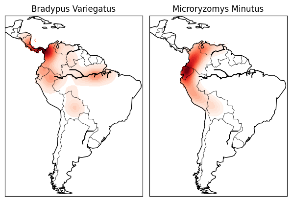
species_names = ['Bradypus Variegatus', 'Microryzomys Minutus']

Xtrain = np.vstack([data['train']['dd lat'],
                    data['train']['dd long']]).T
ytrain = np.array([d.decode('ascii').startswith('micro')
                  for d in data['train']['species']], dtype='int')
Xtrain *= np.pi / 180.  # Convert lat/long to radians

# Set up the data grid for the contour plot
xgrid, ygrid = construct_grids(data)
X, Y = np.meshgrid(xgrid[::5], ygrid[::5][::-1])
land_reference = data.coverages[6][::5, ::5]
land_mask = (land_reference > -9999).ravel()

xy = np.vstack([Y.ravel(), X.ravel()]).T
xy = xy[land_mask]
xy *= np.pi / 180.

# Plot map of South America with distributions of each species
fig = plt.figure()
fig.subplots_adjust(left=0.05, right=0.95, wspace=0.05)

for i in range(2):
    plt.subplot(1, 2, i + 1)

    # construct a kernel density estimate of the distribution
    print(" - computing KDE in spherical coordinates")
    kde = KernelDensity(bandwidth=0.04, metric='haversine',
                        kernel='gaussian', algorithm='ball_tree')
    kde.fit(Xtrain[ytrain == i])

    # evaluate only on the land: -9999 indicates ocean
    Z = np.full(land_mask.shape[0], -9999, dtype='int')
    Z[land_mask] = np.exp(kde.score_samples(xy))
    Z = Z.reshape(X.shape)

    # plot contours of the density
    levels = np.linspace(0, Z.max(), 25)
    plt.contourf(X, Y, Z, levels=levels, cmap=plt.cm.Reds)

    if basemap:
        print(" - plot coastlines using basemap")
        m = Basemap(projection='cyl', llcrnrlat=Y.min(),
                    urcrnrlat=Y.max(), llcrnrlon=X.min(),
                    urcrnrlon=X.max(), resolution='c')
        m.drawcoastlines()
        m.drawcountries()
    else:
        print(" - plot coastlines from coverage")
        plt.contour(X, Y, land_reference,
                    levels=[-9998], colors="k",
                    linestyles="solid")
        plt.xticks([])
        plt.yticks([])

    plt.title(species_names[i])

plt.show()

 - computing KDE in spherical coordinates

 - plot coastlines using basemap
 - computing KDE in spherical coordinates

 - plot coastlines using basemap

k-nearest neighbor estimator

Let \(d_k(x)\) be the minimum radius of an open ball of \(x\) that covers \(k\) points. The k-nearest neighbor density estimate is given by

\[\hat{p}(x) = \frac{k}{2Nd_k(x)}\]

The knn estimator’s derivative has a discontinuity at all \(1/2(x^j+x^{j+k})\). To get a smoother estimator we can use a kernel function

\[\hat{p}(x) = \frac{1}{Nd_k(x)}\sum_{t=1}^Nk\big{(}\frac{x-x^t}{d_k(x)}\big{)}\]

This is a kernel estimator with adaptive smoothing parameter \(h=d_k(x)\). \(k(.)\) is taken to be the Gaussian kernel.

%matplotlib inline
import matplotlib.pyplot as plt
import seaborn as sns; sns.set()
import numpy as np

def make_data(N, f=0.3, rseed=1):
    rand = np.random.RandomState(rseed)
    x = rand.randn(N)
    x[int(f * N):] += 5
    return x

x = make_data(1000)
hist = plt.hist(x, bins=30, density=True)

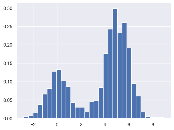
density, bins, patches = hist
widths = bins[1:] - bins[:-1]
(density * widths).sum()

1.0

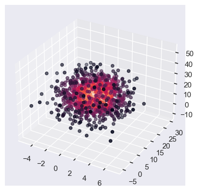
Density estimation for multivariate data

Given a sample of \(p\)-dimensional obvservations \(X=\{x^t\}_{t=1}^N\), the multivariate kernel density estimator is

\[\hat{p}(x) = \frac{1}{Nh^p}\sum_{t=1}^N K\big{(}\frac{x-x^t}{h}\big{)}\]

The kernel is taken to be the multivariate Gaussian kernel

\[K(u) = \big{(}\frac{1}{\sqrt{2\pi}}\big{)}^pexp\big{[}-\frac{||u||^2}{2}\big{]}\]

or

\[K(u) = \frac{1}{(2\pi)^{p/2}|S|^{1/2}}exp\big{[}-\frac{1}{2}u^TS^{-1}u\big{]}\]

where \(S\) is the sample covariance matrix. It is also possible to calculate the local \(S\) from instances in the vicinity of \(x\). If the local \(S\) is singular then PCA may be needed

If the inputs are discrete, we can use Hamming distance, which counts the number of nomatching attributes.

import numpy as np
from scipy import stats
import matplotlib.pyplot as plt
from mpl_toolkits.mplot3d import Axes3D

mu=np.array([1,10,20])
sigma=np.matrix([[4,1,1],[1,25,1],[1,1,100]])
data=np.random.multivariate_normal(mu,sigma,1000)
values = data.T
kde1 = stats.gaussian_kde(values)
density = kde1(values)

fig, ax = plt.subplots(subplot_kw=dict(projection='3d'))
x, y, z = values
ax.scatter(x, y, z, c=density)
plt.show()

Nonparametric classification

The kernel estimator of the class-conditional density \(P(x|C_i)\) is given by

\[\hat{p}(x) = \frac{1}{N_ih^p}\sum_{t=1}^N K\big{(}\frac{x-x^t}{h}\big{)}r_i^t\]

where \(r_i^t\) is an indicator of the assignment of \(x\), i.e., \(r_i^t=1\) if \(x\in C_i\) and \(r_i^t=0\) otherwise. The MLE of the prior density is \(\hat{P}(C_i) = N_i/N\). Thus the discriminant function is given by

\[g_i(x) = \hat{P}(x|C_i)\hat{P}(C_i)=\frac{1}{Nh^p}\sum_{t=1}^N K\big{(}\frac{x-x^t}{h}\big{)}r_i^t\]

For the knn estimator, we have

\[\hat{p}(x) = \frac{k_i}{2N_iV^k(x)}\]

where \(k_i\) is the number of the k nearest neighbors that belong to the class \(C_i\). Then the posterior probablity of the class \(C_i\) is

\[\hat{P}(C_i|x) = \frac{k_i}{k}\]

Nonparametric regression: smoothing models

In regression, given the training set \(X=\{x^t,r^t\}\) where \(r^t\in R\), we assume

\[r^t = g(x^t)+\epsilon\]

We assume that \(g(.)\) is a smooth function. In nonparametric regrssion, we will estimate the function \(g(x)\) locally by the nearby points of \(x\)

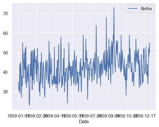
Running mean smoother

The function \(g(x)\) is estimated by the moving average

\[\hat{g}(x) = \frac{\sum_{t=1}^Nw\big{(}\frac{x-x^t}{h}\big{)}r^t}{\sum_{t=1}^{N}w\big{(}\frac{x-x^t}{h}\big{)}}\]

where \(w(u)\) is an indicator function whether the point \(x^t\) is in the neighborhood of \(x\), i.e., \(w(u) = 1\) if \(|u|<1\) and 0 otherwise.

from pandas import read_csv
from matplotlib import pyplot
series = read_csv('https://book.phylolab.net/machine_learning_data/daily-total-female-births.csv', header=0, index_col=0)

print(series.head())
series.plot()
pyplot.show()

            Births
Date              
1959-01-01      35
1959-01-02      32
1959-01-03      30
1959-01-04      31
1959-01-05      44

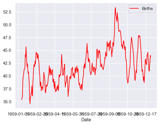
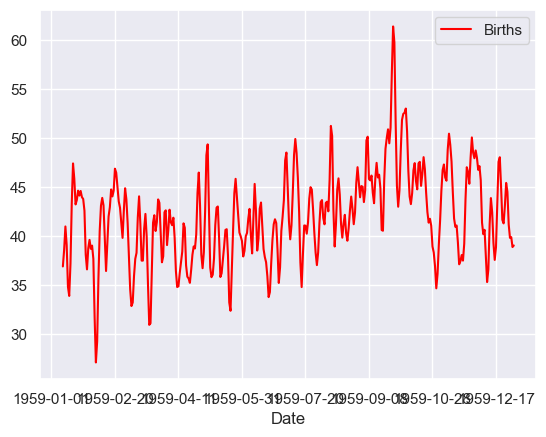
# Tail-rolling average transform
rolling = series.rolling(window=10)
rolling_mean = rolling.mean()
#print(rolling_mean.head(50))
# plot original and transformed dataset
rolling_mean.plot(color='red')
pyplot.show()

Kernel smoother

The function \(g(x)\) is estimated by the moving average

\[\hat{g}(x) = \frac{\sum_{t=1}^NK\big{(}\frac{x-x^t}{h}\big{)}r^t}{\sum_{t=1}^{N}K\big{(}\frac{x-x^t}{h}\big{)}}\]

Typically a Gaussian kernel \(K(.)\) is used. Alternatively, instead of fixing \(h\), we can fix the number of neighbors and getting the knn smoother.

rolling = series.rolling(10, win_type='triang')
rolling_mean = rolling.mean()
rolling_mean.plot(color='red')
pyplot.show()

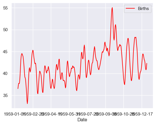
rolling = series.rolling(10, win_type='gaussian')
rolling_mean = rolling.mean(std=1)
rolling_mean.plot(color='red')
pyplot.show()

Running line smoother

Instead of taking an average, we can fit a local linear regression line using the neighbors of \(x\) and then estimate \(g(x)\) from the regression line.

In the locally weighted running line smoother (loess), instead of a hard definition of neighborhoods, we use kernel weighting such that distant points have less effect on error.

How to choose the smoothing parameter

In nonparametric methods, choosing the correct smoothing parameters are important in oversmoothing or undersmoothing problems.

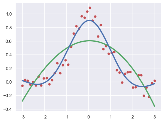
A regularized cost function as used in smoothing splines

\[\sum_t \big{[}r^t -\hat{g}(x^t) \big{]}^2 + \lambda \int_a^b[\hat{g}''(x)]^2dx\]

The first term is the error of fit. The second term \(\hat{g}''(x)\) is the curvature of the estimated function \(\hat{g}(x)\).

import numpy as np
import matplotlib.pyplot as plt
from scipy.interpolate import UnivariateSpline
x = np.linspace(-3, 3, 50)
y = np.exp(-x**2) + 0.1 * np.random.randn(50)
plt.plot(x, y, 'ro', ms=5)

spl = UnivariateSpline(x, y)
xs = np.linspace(-3, 3, 1000)
plt.plot(xs, spl(xs), 'g', lw=3)

spl.set_smoothing_factor(0.5)
plt.plot(xs, spl(xs), 'b', lw=3)
plt.show()