Lab 3: Multivariate Methods#
Parameter Estimation#
Let \(𝑋={𝑋_1,…,𝑋_𝑃}\) be a \(p\)-dimension point. The mean vector is \(\mu=𝐸(𝑋)\) and the covariance matrix is \(Σ_{𝑝×𝑝}\)
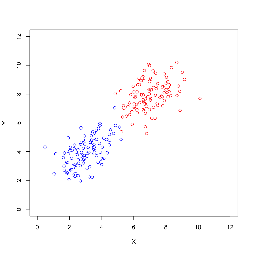
Two normal distributions with different mean and covariance matrix#
library(MASS)
sigma1 = matrix(2,2,2)
sigma1[1,2] = sigma1[2,1]=0.5
bvn1 = mvrnorm(100, mu=c(3,4), Sigma=sigma1)

sigma2 = matrix(1,2,2)
sigma2[1,2] = sigma2[2,1] = 0.5
bvn2 = mvrnorm(100, mu=c(7,8), Sigma=sigma2)

plot(bvn1,xlim=c(0,12),ylim=c(0,12),col="blue",xlab="X",ylab="Y")
points(bvn2,col="red")

The mean vector \(\mu\) can be estimated by the sample average
bvn1_average = apply(bvn1,2,mean)
bvn2_average = apply(bvn2,2,mean)
print("the first group")
bvn1_average
print("the second group")
bvn2_average
[1] "the first group"
- 2.87161703821864
- 3.94169121104734
[1] "the second group"
- 7.11777570362168
- 7.99345609581267
The covariance matrix can be estimated by the sample covariance matrix
bvn1_cov = cov(bvn1)
bvn2_cov = cov(bvn2)

print("the first group")
bvn1_cov
print("the second group")
bvn2_cov
[1] "the first group"
| 2.1131742 | 0.3302313 |
| 0.3302313 | 1.7735052 |
[1] "the second group"
| 0.9037220 | 0.2699806 |
| 0.2699806 | 0.8289249 |
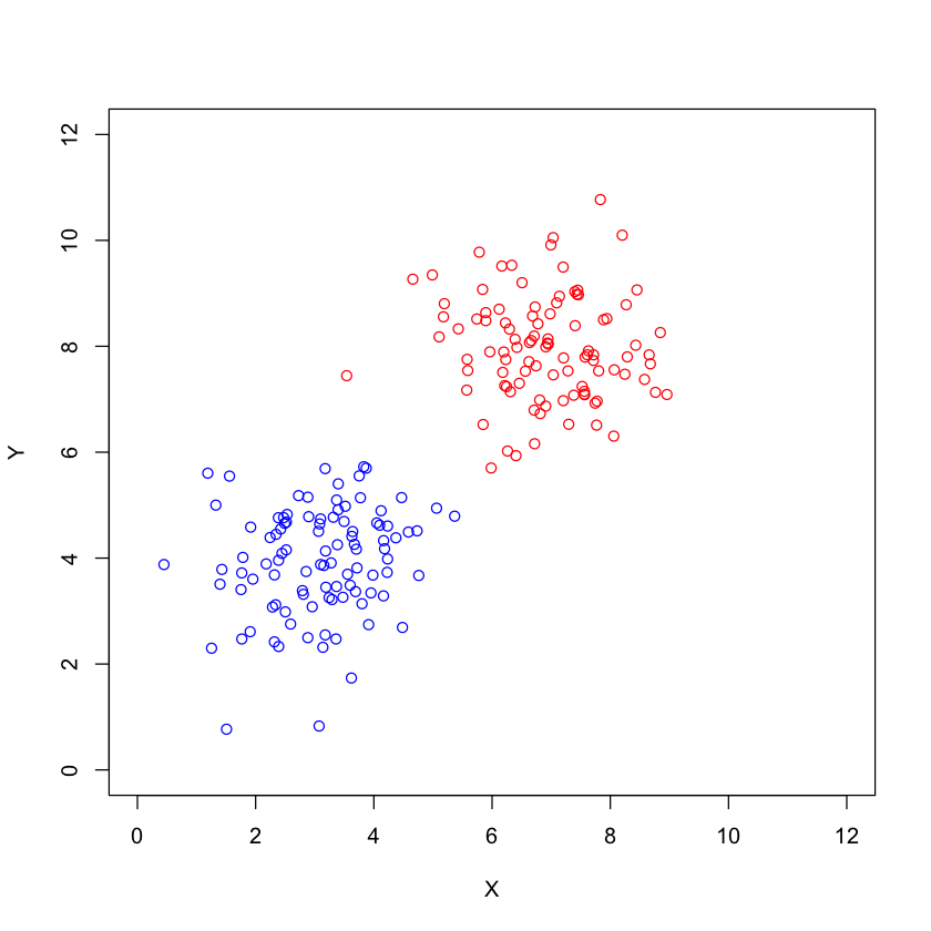
Two classes may have a common covaraince matrix#
sigma = matrix(1,2,2)
sigma[1,2] = sigma[2,1]=0.5

bvn1 = mvrnorm(100, mu=c(3,4), sigma)
bvn2 = mvrnorm(100, mu=c(7,8), sigma)

plot(bvn1,xlim=c(0,12),ylim=c(0,12),col="blue",xlab="X",ylab="Y")
points(bvn2,col="red")
The covariance matrix is estimated by the sample covariance of the pooled data
pooldata = rbind(bvn1-mean(bvn1),bvn2-mean(bvn2))
bvn1_cov = cov(pooldata)

print("The pooled covariance matrix")
bvn1_cov
[1] "The pooled covariance matrix"
| 0.9475637 | 0.4548899 |
| 0.4548899 | 1.0334350 |
Diagnal covariance matrix#
In this case, the coordinate random variables \(X_1,...X_p\) are independently distributed with a normal distribution
sigma = matrix(1,2,2)
sigma[1,2] = sigma[2,1]= 0
sigma[2,2] = 4

bvn1 = mvrnorm(100, mu=c(3,4), sigma)
bvn2 = mvrnorm(100, mu=c(7,8), sigma)

plot(bvn1,xlim=c(0,12),ylim=c(0,12),col="blue",xlab="X",ylab="Y")
points(bvn2,col="red")

Independent random variables with a common variance#
sigma = matrix(1,2,2)
sigma[1,2] = sigma[2,1]= 0

bvn1 = mvrnorm(100, mu=c(3,4), sigma)
bvn2 = mvrnorm(100, mu=c(7,8), sigma)

plot(bvn1,xlim=c(0,12),ylim=c(0,12),col="blue",xlab="X",ylab="Y")
points(bvn2,col="red")
Estimation of Missing Values#
Values of certain variables may be missing in data. For example, the first 10 values of the first column of bvn1 are missing
bvn1[1:10,1] = NA
bvn1
Show code cell output
| NA | 3.342038 |
| NA | 5.142741 |
| NA | 4.449138 |
| NA | 3.683020 |
| NA | 4.620892 |
| NA | 4.383494 |
| NA | 3.983260 |
| NA | 4.329717 |
| NA | 3.719771 |
| NA | 3.890577 |
| 4.1620446 | 3.286794 |
| 2.4238473 | 4.550390 |
| 1.9159840 | 4.585138 |
| 3.3144763 | 4.771536 |
| 2.2444711 | 4.388768 |
| 3.7997688 | 3.138331 |
| 3.0989902 | 3.879268 |
| 4.2320545 | 4.605499 |
| 0.4487672 | 3.878384 |
| 4.7314205 | 4.514621 |
| 3.1831526 | 4.133918 |
| 2.4739274 | 4.764042 |
| 2.7914091 | 3.385800 |
| 4.4837058 | 2.690229 |
| 3.7726170 | 5.139406 |
| 3.6277893 | 4.410551 |
| 2.5915736 | 2.754170 |
| 4.2250190 | 3.730195 |
| 3.6903095 | 3.366985 |
| 1.7657510 | 2.472587 |
| ⋮ | ⋮ |
| 1.784163 | 4.0136187 |
| 3.154825 | 3.8608814 |
| 3.187552 | 3.4497028 |
| 4.759820 | 3.6720317 |
| 4.121890 | 4.8942886 |
| 2.517772 | 4.1546984 |
| 3.073266 | 0.8286488 |
| 3.476263 | 3.2605749 |
| 3.751818 | 5.5526505 |
| 1.557806 | 5.5481571 |
| 3.496160 | 4.6919553 |
| 2.897365 | 4.7821198 |
| 3.828848 | 5.7259362 |
| 3.983346 | 3.6790456 |
| 3.397573 | 5.4021710 |
| 3.359194 | 2.4725090 |
| 2.317347 | 2.4182551 |
| 3.714664 | 3.8142191 |
| 4.180993 | 4.1766792 |
| 3.911623 | 2.7437576 |
| 3.292095 | 3.2170732 |
| 3.176502 | 5.6899334 |
| 3.394305 | 4.9115720 |
| 1.907226 | 2.6100076 |
| 2.726091 | 5.1797545 |
| 4.049758 | 4.6647227 |
| 3.082837 | 4.6455573 |
| 3.619845 | 1.7354289 |
| 1.507648 | 0.7690181 |
| 2.384671 | 4.7626383 |
We fill in the missing entries by estimating them, i.e., imputation. In the main imputation, missing values are replaced by the average of the available data
bvn1[1:10,1] = mean(bvn1[,1],na.rm=T)
bvn1[1:10,1]
- 3.05401879991298
- 3.05401879991298
- 3.05401879991298
- 3.05401879991298
- 3.05401879991298
- 3.05401879991298
- 3.05401879991298
- 3.05401879991298
- 3.05401879991298
- 3.05401879991298
In imputation by regression, missing values are predicted by linear regression
x = bvn1[-(1:10),]
reg = lm(x[,1]~x[,2])
bvn1[1:10,] = reg$coef[1]+bvn1[1:10,2]*reg$coef[2]
bvn1[1:10,1]
- 2.96677099935777
- 3.23452732602819
- 3.13139174297157
- 3.01747345299547
- 3.15693075435671
- 3.12163079969472
- 3.06211776135899
- 3.1136344182391
- 3.02293823082497
- 3.04833624202013
Multivariate Classification#
Let \(\{C_i: i=1,...,k\}\) be the \(k\) classes. The points in the class \(C_i\) follow the multivariate normal distribution with mean vector \(\mu_i\) and covariance matrix \(\Sigma_i\).
Given the training data \(X_i\) in class \(C_i\), the mean vector and covariance matrix can be estimated by the sample average \(\bar{X}_i\) and sample covariance matrix \(S_i\)
sigma1 = matrix(2,2,2)
sigma1[1,2] = sigma1[2,1]=0.5
bvn1 = mvrnorm(100, mu=c(3,4), Sigma=sigma1)

sigma2 = matrix(1,2,2)
sigma2[1,2] = sigma2[2,1] = 0.5
bvn2 = mvrnorm(100, mu=c(7,8), Sigma=sigma2)

bvn1_average = apply(bvn1,2,mean)
bvn2_average = apply(bvn2,2,mean)

bvn1_cov = cov(bvn1)
bvn2_cov = cov(bvn2)
Let \(P(C_i): i=1,...k\) be the prior probabilities of the k classes. Given the training data \(X\), the probablity \(P(C_i)\) can be estimated by the proportion of points in the class \(C_i\)
The Bayes classifier is given by the posterior probability \(g_i(x) = logf(x|C_i) + log(C_i)\). We substitute the mean vector, covariance matrix, and prior probabilties with their estimates. The posterior probability of the class \(C_i\) is
The Bayes classification is that \(x\in C_i\) if \(g_i(x) > g_j(x)\) for \(i,j = 1,...,k\) and \(j\ne i\)
x = rbind(bvn1,bvn2)
g1 = -0.5*diag((x-bvn1_average)%*%solve(bvn1_cov)%*%t(x-bvn1_average))+0.5
g2 = -0.5*diag((x-bvn2_average)%*%solve(bvn2_cov)%*%t(x-bvn2_average))+0.5
print("first class")
which(g1>g2)
print("second class")
which(g1<g2)

print("two misclassified points")
x[which(g1[101:200]>g2[101:200]),]
[1] "first class"
- 1
- 2
- 3
- 4
- 5
- 6
- 7
- 8
- 9
- 10
- 11
- 12
- 13
- 14
- 15
- 16
- 17
- 18
- 19
- 20
- 21
- 22
- 23
- 24
- 25
- 26
- 27
- 28
- 29
- 30
- 31
- 32
- 33
- 34
- 35
- 36
- 37
- 38
- 39
- 40
- 41
- 42
- 43
- 44
- 45
- 46
- 47
- 48
- 49
- 50
- 51
- 52
- 53
- 54
- 55
- 56
- 57
- 58
- 59
- 60
- 61
- 62
- 63
- 64
- 65
- 66
- 67
- 68
- 69
- 70
- 71
- 72
- 73
- 74
- 75
- 76
- 77
- 78
- 79
- 80
- 81
- 82
- 83
- 84
- 85
- 86
- 87
- 88
- 89
- 90
- 92
- 94
- 95
- 96
- 97
- 98
- 99
- 100
- 126
- 133
- 140
- 146
- 166
- 170
- 172
- 180
[1] "second class"
- 91
- 93
- 101
- 102
- 103
- 104
- 105
- 106
- 107
- 108
- 109
- 110
- 111
- 112
- 113
- 114
- 115
- 116
- 117
- 118
- 119
- 120
- 121
- 122
- 123
- 124
- 125
- 127
- 128
- 129
- 130
- 131
- 132
- 134
- 135
- 136
- 137
- 138
- 139
- 141
- 142
- 143
- 144
- 145
- 147
- 148
- 149
- 150
- 151
- 152
- 153
- 154
- 155
- 156
- 157
- 158
- 159
- 160
- 161
- 162
- 163
- 164
- 165
- 167
- 168
- 169
- 171
- 173
- 174
- 175
- 176
- 177
- 178
- 179
- 181
- 182
- 183
- 184
- 185
- 186
- 187
- 188
- 189
- 190
- 191
- 192
- 193
- 194
- 195
- 196
- 197
- 198
- 199
- 200
[1] "two misclassified points"
| 4.212089 | 4.406357 |
| 5.986891 | 2.606797 |
| 3.452428 | 2.750365 |
| 5.175380 | 1.959169 |
| 3.253416 | 4.969929 |
| 4.398661 | 5.682706 |
| 1.928165 | 3.643036 |
| 3.856544 | 5.994505 |
Two classes have a common covariance matrix#
If two classes have a common covariance matrix \(S\), the posterior probability of the class \(C_i\) is
When \(g_i(x)\) is compared with \(g_j(x)\), the quadratic term \(x^TS^{-1}x\) cancels because it is common in all posterior probabilities of classes. Thus, it becomes a linear discriminant
The Bayes classification is that \(x\in C_i\) if \(g_i(x) > g_j(x)\) for \(i,j = 1,...,k\) and \(j\ne i\)
pooldata = rbind(bvn1-mean(bvn1),bvn2-mean(bvn2))
bvn1_cov = bvn2_cov = cov(pooldata)

m1 = 0.5*bvn1_average%*%solve(bvn1_cov)%*%bvn1_average
m2 = 0.5*bvn2_average%*%solve(bvn1_cov)%*%bvn2_average

x = rbind(bvn1,bvn2)
g1 = bvn1_average%*%solve(bvn1_cov)%*%t(x) - c(m1,m1) + 0.5
g2 = bvn2_average%*%solve(bvn2_cov)%*%t(x) - c(m2,m2) + 0.5
print("first class")
which(g1>g2)
print("second class")
which(g1<g2)

print("two misclassified points")
print(x[which(g1[101:200]>g2[101:200]),])
[1] "first class"
- 2
- 3
- 4
- 5
- 6
- 7
- 8
- 9
- 10
- 11
- 12
- 13
- 15
- 16
- 17
- 19
- 20
- 21
- 22
- 23
- 24
- 26
- 27
- 28
- 29
- 30
- 31
- 32
- 33
- 34
- 35
- 36
- 37
- 38
- 39
- 40
- 41
- 42
- 43
- 44
- 45
- 46
- 47
- 48
- 49
- 50
- 51
- 52
- 53
- 54
- 55
- 56
- 57
- 58
- 59
- 60
- 61
- 62
- 63
- 64
- 65
- 66
- 67
- 68
- 69
- 70
- 71
- 72
- 73
- 74
- 75
- 76
- 77
- 78
- 79
- 80
- 81
- 82
- 83
- 84
- 85
- 86
- 87
- 88
- 89
- 90
- 92
- 94
- 95
- 96
- 97
- 98
- 99
- 100
- 163
- 170
- 172
[1] "second class"
- 1
- 14
- 18
- 25
- 91
- 93
- 101
- 102
- 103
- 104
- 105
- 106
- 107
- 108
- 109
- 110
- 111
- 112
- 113
- 114
- 115
- 116
- 117
- 118
- 119
- 120
- 121
- 122
- 123
- 124
- 125
- 126
- 127
- 128
- 129
- 130
- 131
- 132
- 133
- 134
- 135
- 136
- 137
- 138
- 139
- 140
- 141
- 142
- 143
- 144
- 145
- 146
- 147
- 148
- 149
- 150
- 151
- 152
- 153
- 154
- 155
- 156
- 157
- 158
- 159
- 160
- 161
- 162
- 164
- 165
- 166
- 167
- 168
- 169
- 171
- 173
- 174
- 175
- 176
- 177
- 178
- 179
- 180
- 181
- 182
- 183
- 184
- 185
- 186
- 187
- 188
- 189
- 190
- 191
- 192
- 193
- 194
- 195
- 196
- 197
- 198
- 199
- 200
[1] "two misclassified points"
         [,1]     [,2]
[1,] 4.104538 2.824454
[2,] 4.398661 5.682706
[3,] 1.928165 3.643036
Regularized discriminant analysis#
Let \(S_i\) be the sample covaraince matrix for class \(i\) and let \(S\) be the covariance matrix of the pool data. The covariance matrix is written as a weighted average of the three special cases
When \(\lambda=\gamma=0\), it is a quadratic classifier.
When \(\lambda=1\) and \(\gamma=0\), it is a linear classifier.
When \(\lambda=0\) and \(\gamma=1\), the covariance matrices are diagonal with \(\sigma^2\) and it is the nearest mean classifier.
When \(\lambda=1\) and \(\gamma=1\), the covariance matrices are diagonal with the same variance.
The choice of \(\lambda\) and \(\gamma\) can be optimized by cross-validation
library(mlbench)
library(caret)
library(glmnet)
library(klaR)

data(Sonar)
Sonar
Show code cell output
Loading required package: ggplot2
Loading required package: lattice
Loading required package: Matrix
Loaded glmnet 4.1-8
| V1 | V2 | V3 | V4 | V5 | V6 | V7 | V8 | V9 | V10 | ⋯ | V52 | V53 | V54 | V55 | V56 | V57 | V58 | V59 | V60 | Class | |
|---|---|---|---|---|---|---|---|---|---|---|---|---|---|---|---|---|---|---|---|---|---|
| <dbl> | <dbl> | <dbl> | <dbl> | <dbl> | <dbl> | <dbl> | <dbl> | <dbl> | <dbl> | ⋯ | <dbl> | <dbl> | <dbl> | <dbl> | <dbl> | <dbl> | <dbl> | <dbl> | <dbl> | <fct> | |
| 1 | 0.0200 | 0.0371 | 0.0428 | 0.0207 | 0.0954 | 0.0986 | 0.1539 | 0.1601 | 0.3109 | 0.2111 | ⋯ | 0.0027 | 0.0065 | 0.0159 | 0.0072 | 0.0167 | 0.0180 | 0.0084 | 0.0090 | 0.0032 | R |
| 2 | 0.0453 | 0.0523 | 0.0843 | 0.0689 | 0.1183 | 0.2583 | 0.2156 | 0.3481 | 0.3337 | 0.2872 | ⋯ | 0.0084 | 0.0089 | 0.0048 | 0.0094 | 0.0191 | 0.0140 | 0.0049 | 0.0052 | 0.0044 | R |
| 3 | 0.0262 | 0.0582 | 0.1099 | 0.1083 | 0.0974 | 0.2280 | 0.2431 | 0.3771 | 0.5598 | 0.6194 | ⋯ | 0.0232 | 0.0166 | 0.0095 | 0.0180 | 0.0244 | 0.0316 | 0.0164 | 0.0095 | 0.0078 | R |
| 4 | 0.0100 | 0.0171 | 0.0623 | 0.0205 | 0.0205 | 0.0368 | 0.1098 | 0.1276 | 0.0598 | 0.1264 | ⋯ | 0.0121 | 0.0036 | 0.0150 | 0.0085 | 0.0073 | 0.0050 | 0.0044 | 0.0040 | 0.0117 | R |
| 5 | 0.0762 | 0.0666 | 0.0481 | 0.0394 | 0.0590 | 0.0649 | 0.1209 | 0.2467 | 0.3564 | 0.4459 | ⋯ | 0.0031 | 0.0054 | 0.0105 | 0.0110 | 0.0015 | 0.0072 | 0.0048 | 0.0107 | 0.0094 | R |
| 6 | 0.0286 | 0.0453 | 0.0277 | 0.0174 | 0.0384 | 0.0990 | 0.1201 | 0.1833 | 0.2105 | 0.3039 | ⋯ | 0.0045 | 0.0014 | 0.0038 | 0.0013 | 0.0089 | 0.0057 | 0.0027 | 0.0051 | 0.0062 | R |
| 7 | 0.0317 | 0.0956 | 0.1321 | 0.1408 | 0.1674 | 0.1710 | 0.0731 | 0.1401 | 0.2083 | 0.3513 | ⋯ | 0.0201 | 0.0248 | 0.0131 | 0.0070 | 0.0138 | 0.0092 | 0.0143 | 0.0036 | 0.0103 | R |
| 8 | 0.0519 | 0.0548 | 0.0842 | 0.0319 | 0.1158 | 0.0922 | 0.1027 | 0.0613 | 0.1465 | 0.2838 | ⋯ | 0.0081 | 0.0120 | 0.0045 | 0.0121 | 0.0097 | 0.0085 | 0.0047 | 0.0048 | 0.0053 | R |
| 9 | 0.0223 | 0.0375 | 0.0484 | 0.0475 | 0.0647 | 0.0591 | 0.0753 | 0.0098 | 0.0684 | 0.1487 | ⋯ | 0.0145 | 0.0128 | 0.0145 | 0.0058 | 0.0049 | 0.0065 | 0.0093 | 0.0059 | 0.0022 | R |
| 10 | 0.0164 | 0.0173 | 0.0347 | 0.0070 | 0.0187 | 0.0671 | 0.1056 | 0.0697 | 0.0962 | 0.0251 | ⋯ | 0.0090 | 0.0223 | 0.0179 | 0.0084 | 0.0068 | 0.0032 | 0.0035 | 0.0056 | 0.0040 | R |
| 11 | 0.0039 | 0.0063 | 0.0152 | 0.0336 | 0.0310 | 0.0284 | 0.0396 | 0.0272 | 0.0323 | 0.0452 | ⋯ | 0.0062 | 0.0120 | 0.0052 | 0.0056 | 0.0093 | 0.0042 | 0.0003 | 0.0053 | 0.0036 | R |
| 12 | 0.0123 | 0.0309 | 0.0169 | 0.0313 | 0.0358 | 0.0102 | 0.0182 | 0.0579 | 0.1122 | 0.0835 | ⋯ | 0.0133 | 0.0265 | 0.0224 | 0.0074 | 0.0118 | 0.0026 | 0.0092 | 0.0009 | 0.0044 | R |
| 13 | 0.0079 | 0.0086 | 0.0055 | 0.0250 | 0.0344 | 0.0546 | 0.0528 | 0.0958 | 0.1009 | 0.1240 | ⋯ | 0.0176 | 0.0127 | 0.0088 | 0.0098 | 0.0019 | 0.0059 | 0.0058 | 0.0059 | 0.0032 | R |
| 14 | 0.0090 | 0.0062 | 0.0253 | 0.0489 | 0.1197 | 0.1589 | 0.1392 | 0.0987 | 0.0955 | 0.1895 | ⋯ | 0.0059 | 0.0095 | 0.0194 | 0.0080 | 0.0152 | 0.0158 | 0.0053 | 0.0189 | 0.0102 | R |
| 15 | 0.0124 | 0.0433 | 0.0604 | 0.0449 | 0.0597 | 0.0355 | 0.0531 | 0.0343 | 0.1052 | 0.2120 | ⋯ | 0.0083 | 0.0057 | 0.0174 | 0.0188 | 0.0054 | 0.0114 | 0.0196 | 0.0147 | 0.0062 | R |
| 16 | 0.0298 | 0.0615 | 0.0650 | 0.0921 | 0.1615 | 0.2294 | 0.2176 | 0.2033 | 0.1459 | 0.0852 | ⋯ | 0.0031 | 0.0153 | 0.0071 | 0.0212 | 0.0076 | 0.0152 | 0.0049 | 0.0200 | 0.0073 | R |
| 17 | 0.0352 | 0.0116 | 0.0191 | 0.0469 | 0.0737 | 0.1185 | 0.1683 | 0.1541 | 0.1466 | 0.2912 | ⋯ | 0.0346 | 0.0158 | 0.0154 | 0.0109 | 0.0048 | 0.0095 | 0.0015 | 0.0073 | 0.0067 | R |
| 18 | 0.0192 | 0.0607 | 0.0378 | 0.0774 | 0.1388 | 0.0809 | 0.0568 | 0.0219 | 0.1037 | 0.1186 | ⋯ | 0.0331 | 0.0131 | 0.0120 | 0.0108 | 0.0024 | 0.0045 | 0.0037 | 0.0112 | 0.0075 | R |
| 19 | 0.0270 | 0.0092 | 0.0145 | 0.0278 | 0.0412 | 0.0757 | 0.1026 | 0.1138 | 0.0794 | 0.1520 | ⋯ | 0.0084 | 0.0010 | 0.0018 | 0.0068 | 0.0039 | 0.0120 | 0.0132 | 0.0070 | 0.0088 | R |
| 20 | 0.0126 | 0.0149 | 0.0641 | 0.1732 | 0.2565 | 0.2559 | 0.2947 | 0.4110 | 0.4983 | 0.5920 | ⋯ | 0.0092 | 0.0035 | 0.0098 | 0.0121 | 0.0006 | 0.0181 | 0.0094 | 0.0116 | 0.0063 | R |
| 21 | 0.0473 | 0.0509 | 0.0819 | 0.1252 | 0.1783 | 0.3070 | 0.3008 | 0.2362 | 0.3830 | 0.3759 | ⋯ | 0.0193 | 0.0118 | 0.0064 | 0.0042 | 0.0054 | 0.0049 | 0.0082 | 0.0028 | 0.0027 | R |
| 22 | 0.0664 | 0.0575 | 0.0842 | 0.0372 | 0.0458 | 0.0771 | 0.0771 | 0.1130 | 0.2353 | 0.1838 | ⋯ | 0.0141 | 0.0190 | 0.0043 | 0.0036 | 0.0026 | 0.0024 | 0.0162 | 0.0109 | 0.0079 | R |
| 23 | 0.0099 | 0.0484 | 0.0299 | 0.0297 | 0.0652 | 0.1077 | 0.2363 | 0.2385 | 0.0075 | 0.1882 | ⋯ | 0.0173 | 0.0149 | 0.0115 | 0.0202 | 0.0139 | 0.0029 | 0.0160 | 0.0106 | 0.0134 | R |
| 24 | 0.0115 | 0.0150 | 0.0136 | 0.0076 | 0.0211 | 0.1058 | 0.1023 | 0.0440 | 0.0931 | 0.0734 | ⋯ | 0.0091 | 0.0016 | 0.0084 | 0.0064 | 0.0026 | 0.0029 | 0.0037 | 0.0070 | 0.0041 | R |
| 25 | 0.0293 | 0.0644 | 0.0390 | 0.0173 | 0.0476 | 0.0816 | 0.0993 | 0.0315 | 0.0736 | 0.0860 | ⋯ | 0.0035 | 0.0052 | 0.0083 | 0.0078 | 0.0075 | 0.0105 | 0.0160 | 0.0095 | 0.0011 | R |
| 26 | 0.0201 | 0.0026 | 0.0138 | 0.0062 | 0.0133 | 0.0151 | 0.0541 | 0.0210 | 0.0505 | 0.1097 | ⋯ | 0.0108 | 0.0070 | 0.0063 | 0.0030 | 0.0011 | 0.0007 | 0.0024 | 0.0057 | 0.0044 | R |
| 27 | 0.0151 | 0.0320 | 0.0599 | 0.1050 | 0.1163 | 0.1734 | 0.1679 | 0.1119 | 0.0889 | 0.1205 | ⋯ | 0.0061 | 0.0015 | 0.0084 | 0.0128 | 0.0054 | 0.0011 | 0.0019 | 0.0023 | 0.0062 | R |
| 28 | 0.0177 | 0.0300 | 0.0288 | 0.0394 | 0.0630 | 0.0526 | 0.0688 | 0.0633 | 0.0624 | 0.0613 | ⋯ | 0.0102 | 0.0122 | 0.0044 | 0.0075 | 0.0124 | 0.0099 | 0.0057 | 0.0032 | 0.0019 | R |
| 29 | 0.0100 | 0.0275 | 0.0190 | 0.0371 | 0.0416 | 0.0201 | 0.0314 | 0.0651 | 0.1896 | 0.2668 | ⋯ | 0.0088 | 0.0104 | 0.0036 | 0.0088 | 0.0047 | 0.0117 | 0.0020 | 0.0091 | 0.0058 | R |
| 30 | 0.0189 | 0.0308 | 0.0197 | 0.0622 | 0.0080 | 0.0789 | 0.1440 | 0.1451 | 0.1789 | 0.2522 | ⋯ | 0.0038 | 0.0096 | 0.0142 | 0.0190 | 0.0140 | 0.0099 | 0.0092 | 0.0052 | 0.0075 | R |
| ⋮ | ⋮ | ⋮ | ⋮ | ⋮ | ⋮ | ⋮ | ⋮ | ⋮ | ⋮ | ⋮ | ⋱ | ⋮ | ⋮ | ⋮ | ⋮ | ⋮ | ⋮ | ⋮ | ⋮ | ⋮ | ⋮ |
| 179 | 0.0197 | 0.0394 | 0.0384 | 0.0076 | 0.0251 | 0.0629 | 0.0747 | 0.0578 | 0.1357 | 0.1695 | ⋯ | 0.0134 | 0.0097 | 0.0042 | 0.0058 | 0.0072 | 0.0041 | 0.0045 | 0.0047 | 0.0054 | M |
| 180 | 0.0394 | 0.0420 | 0.0446 | 0.0551 | 0.0597 | 0.1416 | 0.0956 | 0.0802 | 0.1618 | 0.2558 | ⋯ | 0.0146 | 0.0040 | 0.0114 | 0.0032 | 0.0062 | 0.0101 | 0.0068 | 0.0053 | 0.0087 | M |
| 181 | 0.0310 | 0.0221 | 0.0433 | 0.0191 | 0.0964 | 0.1827 | 0.1106 | 0.1702 | 0.2804 | 0.4432 | ⋯ | 0.0204 | 0.0059 | 0.0053 | 0.0079 | 0.0037 | 0.0015 | 0.0056 | 0.0067 | 0.0054 | M |
| 182 | 0.0423 | 0.0321 | 0.0709 | 0.0108 | 0.1070 | 0.0973 | 0.0961 | 0.1323 | 0.2462 | 0.2696 | ⋯ | 0.0176 | 0.0035 | 0.0093 | 0.0121 | 0.0075 | 0.0056 | 0.0021 | 0.0043 | 0.0017 | M |
| 183 | 0.0095 | 0.0308 | 0.0539 | 0.0411 | 0.0613 | 0.1039 | 0.1016 | 0.1394 | 0.2592 | 0.3745 | ⋯ | 0.0181 | 0.0019 | 0.0102 | 0.0133 | 0.0040 | 0.0042 | 0.0030 | 0.0031 | 0.0033 | M |
| 184 | 0.0096 | 0.0404 | 0.0682 | 0.0688 | 0.0887 | 0.0932 | 0.0955 | 0.2140 | 0.2546 | 0.2952 | ⋯ | 0.0237 | 0.0078 | 0.0144 | 0.0170 | 0.0012 | 0.0109 | 0.0036 | 0.0043 | 0.0018 | M |
| 185 | 0.0269 | 0.0383 | 0.0505 | 0.0707 | 0.1313 | 0.2103 | 0.2263 | 0.2524 | 0.3595 | 0.5915 | ⋯ | 0.0167 | 0.0199 | 0.0145 | 0.0081 | 0.0045 | 0.0043 | 0.0027 | 0.0055 | 0.0057 | M |
| 186 | 0.0340 | 0.0625 | 0.0381 | 0.0257 | 0.0441 | 0.1027 | 0.1287 | 0.1850 | 0.2647 | 0.4117 | ⋯ | 0.0141 | 0.0019 | 0.0067 | 0.0099 | 0.0042 | 0.0057 | 0.0051 | 0.0033 | 0.0058 | M |
| 187 | 0.0209 | 0.0191 | 0.0411 | 0.0321 | 0.0698 | 0.1579 | 0.1438 | 0.1402 | 0.3048 | 0.3914 | ⋯ | 0.0078 | 0.0201 | 0.0104 | 0.0039 | 0.0031 | 0.0062 | 0.0087 | 0.0070 | 0.0042 | M |
| 188 | 0.0368 | 0.0279 | 0.0103 | 0.0566 | 0.0759 | 0.0679 | 0.0970 | 0.1473 | 0.2164 | 0.2544 | ⋯ | 0.0105 | 0.0024 | 0.0018 | 0.0057 | 0.0092 | 0.0009 | 0.0086 | 0.0110 | 0.0052 | M |
| 189 | 0.0089 | 0.0274 | 0.0248 | 0.0237 | 0.0224 | 0.0845 | 0.1488 | 0.1224 | 0.1569 | 0.2119 | ⋯ | 0.0096 | 0.0103 | 0.0093 | 0.0025 | 0.0044 | 0.0021 | 0.0069 | 0.0060 | 0.0018 | M |
| 190 | 0.0158 | 0.0239 | 0.0150 | 0.0494 | 0.0988 | 0.1425 | 0.1463 | 0.1219 | 0.1697 | 0.1923 | ⋯ | 0.0121 | 0.0108 | 0.0057 | 0.0028 | 0.0079 | 0.0034 | 0.0046 | 0.0022 | 0.0021 | M |
| 191 | 0.0156 | 0.0210 | 0.0282 | 0.0596 | 0.0462 | 0.0779 | 0.1365 | 0.0780 | 0.1038 | 0.1567 | ⋯ | 0.0150 | 0.0060 | 0.0082 | 0.0091 | 0.0038 | 0.0056 | 0.0056 | 0.0048 | 0.0024 | M |
| 192 | 0.0315 | 0.0252 | 0.0167 | 0.0479 | 0.0902 | 0.1057 | 0.1024 | 0.1209 | 0.1241 | 0.1533 | ⋯ | 0.0108 | 0.0062 | 0.0044 | 0.0072 | 0.0007 | 0.0054 | 0.0035 | 0.0001 | 0.0055 | M |
| 193 | 0.0056 | 0.0267 | 0.0221 | 0.0561 | 0.0936 | 0.1146 | 0.0706 | 0.0996 | 0.1673 | 0.1859 | ⋯ | 0.0072 | 0.0055 | 0.0074 | 0.0068 | 0.0084 | 0.0037 | 0.0024 | 0.0034 | 0.0007 | M |
| 194 | 0.0203 | 0.0121 | 0.0380 | 0.0128 | 0.0537 | 0.0874 | 0.1021 | 0.0852 | 0.1136 | 0.1747 | ⋯ | 0.0134 | 0.0094 | 0.0047 | 0.0045 | 0.0042 | 0.0028 | 0.0036 | 0.0013 | 0.0016 | M |
| 195 | 0.0392 | 0.0108 | 0.0267 | 0.0257 | 0.0410 | 0.0491 | 0.1053 | 0.1690 | 0.2105 | 0.2471 | ⋯ | 0.0083 | 0.0080 | 0.0026 | 0.0079 | 0.0042 | 0.0071 | 0.0044 | 0.0022 | 0.0014 | M |
| 196 | 0.0129 | 0.0141 | 0.0309 | 0.0375 | 0.0767 | 0.0787 | 0.0662 | 0.1108 | 0.1777 | 0.2245 | ⋯ | 0.0124 | 0.0093 | 0.0072 | 0.0019 | 0.0027 | 0.0054 | 0.0017 | 0.0024 | 0.0029 | M |
| 197 | 0.0050 | 0.0017 | 0.0270 | 0.0450 | 0.0958 | 0.0830 | 0.0879 | 0.1220 | 0.1977 | 0.2282 | ⋯ | 0.0165 | 0.0056 | 0.0010 | 0.0027 | 0.0062 | 0.0024 | 0.0063 | 0.0017 | 0.0028 | M |
| 198 | 0.0366 | 0.0421 | 0.0504 | 0.0250 | 0.0596 | 0.0252 | 0.0958 | 0.0991 | 0.1419 | 0.1847 | ⋯ | 0.0132 | 0.0027 | 0.0022 | 0.0059 | 0.0016 | 0.0025 | 0.0017 | 0.0027 | 0.0027 | M |
| 199 | 0.0238 | 0.0318 | 0.0422 | 0.0399 | 0.0788 | 0.0766 | 0.0881 | 0.1143 | 0.1594 | 0.2048 | ⋯ | 0.0096 | 0.0071 | 0.0084 | 0.0038 | 0.0026 | 0.0028 | 0.0013 | 0.0035 | 0.0060 | M |
| 200 | 0.0116 | 0.0744 | 0.0367 | 0.0225 | 0.0076 | 0.0545 | 0.1110 | 0.1069 | 0.1708 | 0.2271 | ⋯ | 0.0141 | 0.0103 | 0.0100 | 0.0034 | 0.0026 | 0.0037 | 0.0044 | 0.0057 | 0.0035 | M |
| 201 | 0.0131 | 0.0387 | 0.0329 | 0.0078 | 0.0721 | 0.1341 | 0.1626 | 0.1902 | 0.2610 | 0.3193 | ⋯ | 0.0150 | 0.0076 | 0.0032 | 0.0037 | 0.0071 | 0.0040 | 0.0009 | 0.0015 | 0.0085 | M |
| 202 | 0.0335 | 0.0258 | 0.0398 | 0.0570 | 0.0529 | 0.1091 | 0.1709 | 0.1684 | 0.1865 | 0.2660 | ⋯ | 0.0120 | 0.0039 | 0.0053 | 0.0062 | 0.0046 | 0.0045 | 0.0022 | 0.0005 | 0.0031 | M |
| 203 | 0.0272 | 0.0378 | 0.0488 | 0.0848 | 0.1127 | 0.1103 | 0.1349 | 0.2337 | 0.3113 | 0.3997 | ⋯ | 0.0091 | 0.0045 | 0.0043 | 0.0043 | 0.0098 | 0.0054 | 0.0051 | 0.0065 | 0.0103 | M |
| 204 | 0.0187 | 0.0346 | 0.0168 | 0.0177 | 0.0393 | 0.1630 | 0.2028 | 0.1694 | 0.2328 | 0.2684 | ⋯ | 0.0116 | 0.0098 | 0.0199 | 0.0033 | 0.0101 | 0.0065 | 0.0115 | 0.0193 | 0.0157 | M |
| 205 | 0.0323 | 0.0101 | 0.0298 | 0.0564 | 0.0760 | 0.0958 | 0.0990 | 0.1018 | 0.1030 | 0.2154 | ⋯ | 0.0061 | 0.0093 | 0.0135 | 0.0063 | 0.0063 | 0.0034 | 0.0032 | 0.0062 | 0.0067 | M |
| 206 | 0.0522 | 0.0437 | 0.0180 | 0.0292 | 0.0351 | 0.1171 | 0.1257 | 0.1178 | 0.1258 | 0.2529 | ⋯ | 0.0160 | 0.0029 | 0.0051 | 0.0062 | 0.0089 | 0.0140 | 0.0138 | 0.0077 | 0.0031 | M |
| 207 | 0.0303 | 0.0353 | 0.0490 | 0.0608 | 0.0167 | 0.1354 | 0.1465 | 0.1123 | 0.1945 | 0.2354 | ⋯ | 0.0086 | 0.0046 | 0.0126 | 0.0036 | 0.0035 | 0.0034 | 0.0079 | 0.0036 | 0.0048 | M |
| 208 | 0.0260 | 0.0363 | 0.0136 | 0.0272 | 0.0214 | 0.0338 | 0.0655 | 0.1400 | 0.1843 | 0.2354 | ⋯ | 0.0146 | 0.0129 | 0.0047 | 0.0039 | 0.0061 | 0.0040 | 0.0036 | 0.0061 | 0.0115 | M |
Regularized Discriminant Analysis
set.seed(1337)
cv_5_grid = trainControl(method = "cv", number = 5)
fit_rda_grid = train(Class ~ ., data = Sonar, method = "rda", trControl = cv_5_grid)
fit_rda_grid
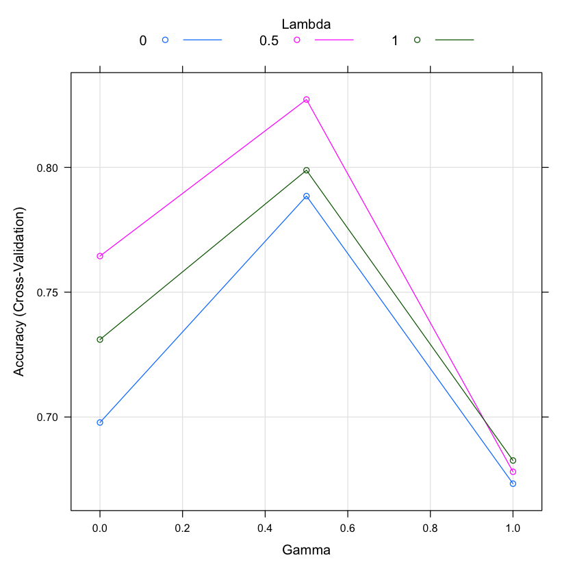
plot(fit_rda_grid)
Regularized Discriminant Analysis

208 samples
 60 predictor
  2 classes: 'M', 'R'

No pre-processing
Resampling: Cross-Validated (5 fold)
Summary of sample sizes: 167, 166, 166, 167, 166
Resampling results across tuning parameters:

  gamma  lambda  Accuracy   Kappa
  0.0    0.0     0.6977933  0.3791172
  0.0    0.5     0.7644599  0.5259800
  0.0    1.0     0.7310105  0.4577198
  0.5    0.0     0.7885017  0.5730052
  0.5    0.5     0.8271777  0.6502693
  0.5    1.0     0.7988386  0.5939209
  1.0    0.0     0.6732869  0.3418352
  1.0    0.5     0.6780488  0.3527778
  1.0    1.0     0.6825784  0.3631626

Accuracy was used to select the optimal model using the largest value.
The final values used for the model were gamma = 0.5 and lambda = 0.5.