Lab 14: Applications

Application 1 - Visualizing face data

We apply Isomap on some faces data. Running this command will download the data and cache it in your home directory for later use. We have 2,370 images, each with 2,914 pixels. In other words, the images can be thought of as data points in a 2,914-dimensional space!

%matplotlib inline
import matplotlib.pyplot as plt
import numpy as np
from sklearn.datasets import fetch_lfw_people

faces = fetch_lfw_people(min_faces_per_person=40)
faces.data.shape

(1867, 2914)

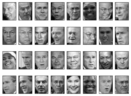
Let’s quickly visualize several of these images to see what we’re working with:

fig, ax = plt.subplots(4, 8, subplot_kw=dict(xticks=[], yticks=[]))
for i, axi in enumerate(ax.flat):
    axi.imshow(faces.images[i], cmap='gray')

We would like to plot a low-dimensional embedding of the 2,914-dimensional data to learn the fundamental relationships between the images. One useful way to start is to compute a PCA, and examine the explained variance ratio, which will give us an idea of how many linear features are required to describe the data:

from sklearn.decomposition import PCA as RandomizedPCA
model = RandomizedPCA(100).fit(faces.data)
plt.plot(np.cumsum(model.explained_variance_ratio_))
plt.xlabel('n components')
plt.ylabel('cumulative variance');

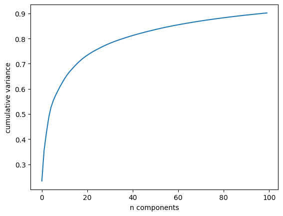
We see that for this data, nearly 100 components are required to preserve 90% of the variance: this tells us that the data is intrinsically very high dimensional—it can’t be described linearly with just a few components.

When this is the case, nonlinear manifold embeddings like LLE and Isomap can be helpful. We can compute an Isomap embedding on these faces using the same pattern shown before:

from sklearn.manifold import Isomap
model = Isomap(n_components=2)
proj = model.fit_transform(faces.data)
proj.shape

(1867, 2)

The output is a two-dimensional projection of all the input images. To get a better idea of what the projection tells us, let’s define a function that will output image thumbnails at the locations of the projections:

from matplotlib import offsetbox

def plot_components(data, model, images=None, ax=None,
                    thumb_frac=0.05, cmap='gray'):
    ax = ax or plt.gca()
    
    proj = model.fit_transform(data)
    ax.plot(proj[:, 0], proj[:, 1], '.k')
    
    if images is not None:
        min_dist_2 = (thumb_frac * max(proj.max(0) - proj.min(0))) ** 2
        shown_images = np.array([2 * proj.max(0)])
        for i in range(data.shape[0]):
            dist = np.sum((proj[i] - shown_images) ** 2, 1)
            if np.min(dist) < min_dist_2:
                # don't show points that are too close
                continue
            shown_images = np.vstack([shown_images, proj[i]])
            imagebox = offsetbox.AnnotationBbox(
                offsetbox.OffsetImage(images[i], cmap=cmap),
                                      proj[i])
            ax.add_artist(imagebox)

Calling this function now, we see the result:

fig, ax = plt.subplots(figsize=(10, 10))
plot_components(faces.data,
                model=Isomap(n_components=2),
                images=faces.images[:, ::2, ::2])

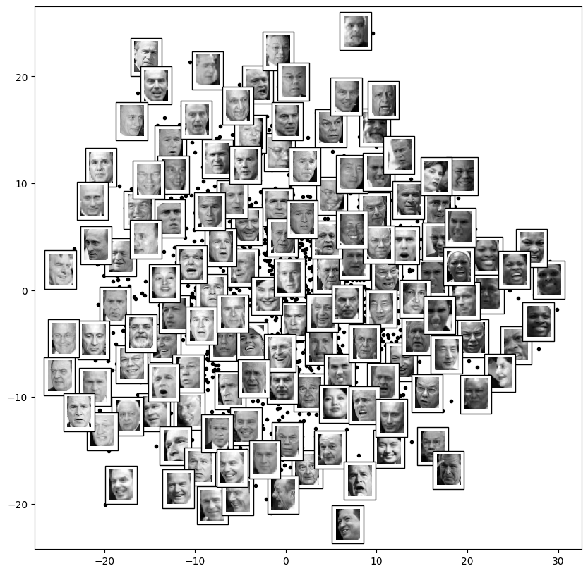
The result is interesting: the first two Isomap dimensions seem to describe global image features: the overall darkness or lightness of the image from left to right, and the general orientation of the face from bottom to top. This gives us a nice visual indication of some of the fundamental features in our data.

We could then go on to classify this data (perhaps using manifold features as inputs to the classification algorithm) as we did in In-Depth: Support Vector Machines.