Simulating Stochastic Processes

1. Discrete time Markov Chain with finite state space

Let \(\pi_t\) be the probability distribution at time t where \(t = 0, 1, 2, \dots\). Let \(\mathbb{P}\) be the \(n\times n\) one step transition probability matrix. By the Komolgorov-Chapman theorem, \(\pi_{t+1} = \pi_t\mathbb{P}\) and

\[\pi_t = \pi_0\mathbb{P}^t\]

The limiting probability \(\pi_\infty = \pi_\infty\mathbb{P}\). Thus, \(\pi_\infty\) is the eigen vector of \(\mathbb{P}^{'}\) for eigen value = 1.

Specify the states of the process

states = c("ATLANTA","CHICAGO","DC","NYC")
nstates = length(states)

Initial Probability at time 0

pi_0 = c(1,0,0,0)

Transition Probability Matrix

tranP = matrix(runif(nstates*nstates),nrow=nstates,ncol=nstates)
for(i in 1:nstates) tranP[i,] = tranP[i,]/sum(tranP[i,])

The Probability distribution at time n

ntime = 20
pi_n = matrix(0,nrow=ntime,ncol=nstates)
tranP_n = diag(nstates)

for(n in 1:ntime){
    tranP_n = tranP %*% tranP_n
    pi_n[n,] = pi_0 %*% tranP_n
}

print("the probablity distribution at time n")
pi_n

print("the n-step transition probability matrix")
tranP_n

[1] "the probablity distribution at time n"

A matrix: 20 × 4 of type dbl

0.3066354	0.02105562	0.3324078	0.3399012
0.2656204	0.29521431	0.2402948	0.1988705
0.2930223	0.30675994	0.1886556	0.2115622
0.3075557	0.29526546	0.1867387	0.2104401
0.3070263	0.28971512	0.1905945	0.2126641
0.3059295	0.29003745	0.1916032	0.2124299
0.3056883	0.29047424	0.1914708	0.2123666
0.3057459	0.29056129	0.1913586	0.2123342
0.3057757	0.29053635	0.1913462	0.2123417
0.3057776	0.29052488	0.1913534	0.2123441
0.3057753	0.29052437	0.1913560	0.2123444
0.3057747	0.29052532	0.1913559	0.2123441
0.3057747	0.29052554	0.1913556	0.2123441
0.3057748	0.29052551	0.1913556	0.2123441
0.3057748	0.29052549	0.1913556	0.2123441
0.3057748	0.29052548	0.1913556	0.2123441
0.3057748	0.29052548	0.1913556	0.2123441
0.3057748	0.29052549	0.1913556	0.2123441
0.3057748	0.29052549	0.1913556	0.2123441
0.3057748	0.29052549	0.1913556	0.2123441

[1] "the n-step transition probability matrix"

A matrix: 4 × 4 of type dbl

0.3057748	0.2905255	0.1913556	0.2123441
0.3057748	0.2905255	0.1913556	0.2123441
0.3057748	0.2905255	0.1913556	0.2123441
0.3057748	0.2905255	0.1913556	0.2123441

Limiting probability distribution

pi = eigen(t(tranP))$vector[,1]
pi = pi/sum(pi)
pi

1. 0.305774795884444+0i
2. 0.290525485078612+0i
3. 0.191355614662356+0i
4. 0.212344104374588+0i

Simulation

nsim = 50
x = rep(0,nsim)
x[1] = sample(1:nstates,1,prob = pi_0)
for(i in 2:nsim){
    x[i] = sample(1:nstates,1,prob = tranP[x[i-1],])
}

freq = table(states[x])
freq/sum(freq)

plot(1:nsim, x, xlab="time", ylab="state", type="l")
                  

ATLANTA CHICAGO      DC     NYC 
   0.24    0.34    0.24    0.18 

Animation

data = rbind(c(1,1),c(2,2),c(2,0),c(3,1))
data = data[x,]

library(plotly)

df <- data.frame(
  x = data[,1], 
  y = data[,2], 
  f = 1:nsim,
  s = states[x]
)

fig <- df %>%
  plot_ly(
    x = ~x,
    y = ~y,
    frame = ~f,
    type = 'scatter',
    mode = 'markers',
    color = I("blue"),
    size = I(50)
  )

t <- list(
  family = "sans serif",
  size = 18,
  color = toRGB("red"))

fig <- fig %>% add_text(x = data[,1],y=data[,2],text = states[x],textfont=t,textposition="top right")
fig <- fig %>% layout(xaxis = list(range = c(0, 4)), yaxis = list(range = c(0,3)), showlegend = FALSE)

fig

Error in library(plotly): there is no package called ‘plotly’
Traceback:

1. library(plotly)

2. Ransom walks

A random walk is a Markov chain with infinite state space. Let \(\pi_t\) be the probability distribution at time \(t\). Let be the \(n\times n\) one step transition probability matrix \(\mathbb{P}\). The Kolmogorov-Chapman theorem still holds, i.e.,

\[\pi_{t+1} = \pi_t\mathbb{P}\]

This indicates that \(\pi_{t+1}^i = \pi_t^{i-1}\times q + \pi_t^{i+1}\times p\)

Initial probability distribution

x[1] = 0

Transition probability

tranP = function(current,p){
    return(ifelse(runif(1)<=p,current-1,current+1))
}

y = 1:10000
for(i in 1:10000) y[i] = tranP(3,0.5)
sum(y==2)

4980

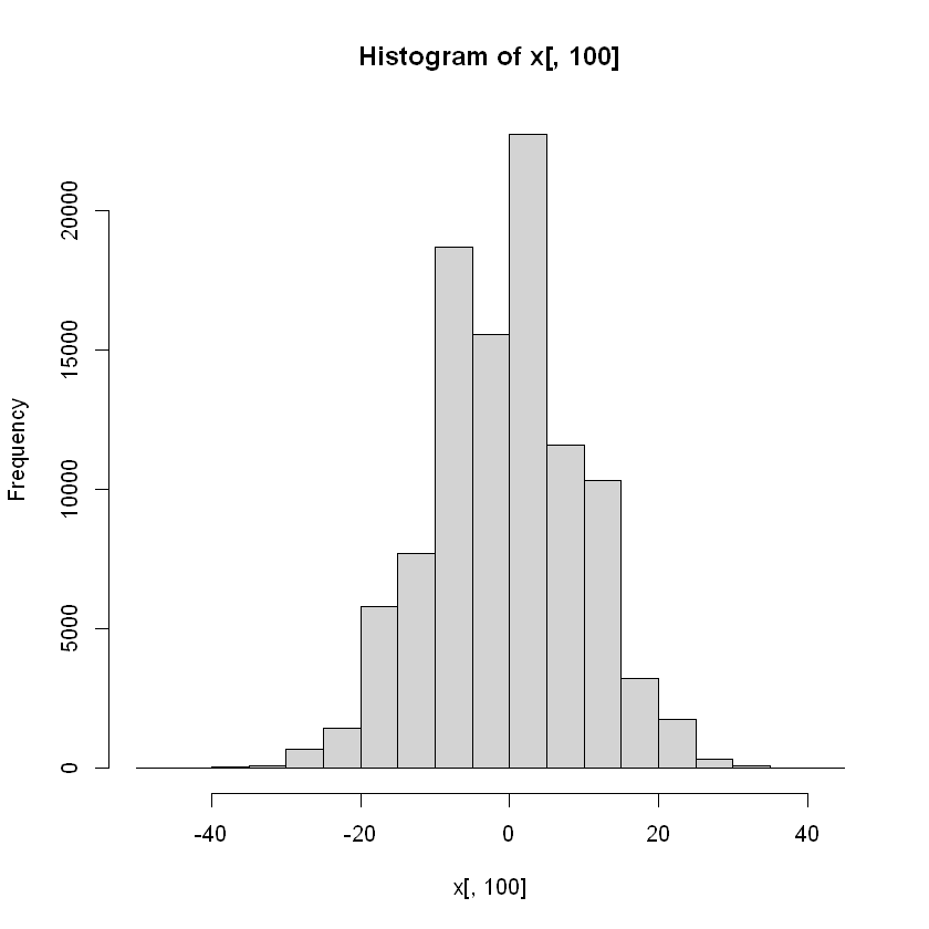
Simulation

nsim = 1000
t = 100
p = 0.5
x = matrix(0, nsim, t)
for(j in 1:nsim){
    for(i in 2:t){
        x[j,i] = tranP(x[j,i-1],p)
    }
}

hist(x[,100])